
This is perhaps the best known database to be found in the pattern recognition literature. Fisher’s paper is a classic in the field and is referenced frequently to this day. (See Duda & Hart, for example.) The data set contains 3 classes of 50 instances each, where each class refers to a type of iris plant. One class is linearly separable from the other 2; the latter are NOT linearly separable from each other.
Predicted attribute: class of iris plant.
This is an exceedingly simple domain.
Our goal is to build a machine learning model that can learn from the measurements of these irises whose species is known, so that we can predict the species for a new
iris.
Because we have measurements for which we know the correct species of iris, this is a supervised learning problem. In this problem, we want to predict one of several
options (the species of iris). This is an example of a classification problem. The possible outputs (different species of irises) are called classes. Every iris in the dataset belongs to one of three classes, so this problem is a three-class classification problem. The desired output for a single data point (an iris) is the species of this flower. For a particular data point, the species it belongs to is called its label.
Loading the Data
The data we will use for this example is the Iris dataset, a classical dataset in machine learning and statistics. It is included in scikit-learn in the datasets module. We can load it by calling the load_iris function:
from sklearn.datasets import load_iris
iris_dataset = load_iris()

print("Keys of iris_dataset:\n", iris_dataset.keys())
Keys of iris_dataset:
 dict_keys(['data', 'target', 'frame', 'target_names', 'DESCR', 'feature_names', 'filename', 'data_module'])
print("Target names:", iris_dataset['target_names'])
print("Feature names:\n", iris_dataset['feature_names'])
Target names: ['setosa' 'versicolor' 'virginica']
Feature names:
 ['sepal length (cm)', 'sepal width (cm)', 'petal length (cm)', 'petal width (cm)']
print("Type of data:", type(iris_dataset['data']))

print("Shape of data:", iris_dataset['data'].shape)
print("Shape of target: {}".format(iris_dataset['target'].shape))
Type of data: <class 'numpy.ndarray'>
Shape of data: (150, 4)
Shape of target: (150,)
We see that the array contains measurements for 150 different flowers. target is a one-dimensional array, with one entry per flower.
print("Target:\n{}".format(iris_dataset['target']))
Target:
[0 0 0 0 0 0 0 0 0 0 0 0 0 0 0 0 0 0 0 0 0 0 0 0 0 0 0 0 0 0 0 0 0 0 0 0 0
 0 0 0 0 0 0 0 0 0 0 0 0 0 1 1 1 1 1 1 1 1 1 1 1 1 1 1 1 1 1 1 1 1 1 1 1 1
 1 1 1 1 1 1 1 1 1 1 1 1 1 1 1 1 1 1 1 1 1 1 1 1 1 1 2 2 2 2 2 2 2 2 2 2 2
 2 2 2 2 2 2 2 2 2 2 2 2 2 2 2 2 2 2 2 2 2 2 2 2 2 2 2 2 2 2 2 2 2 2 2 2 2
 2 2]
0 means setosa, 1 means versicolor, and 2 means virginica.
Training and Testing Data
First, we need to assess the model performance. we show it new data (data that it hasn’t seen before) for which we have labels. This is usually done by splitting the labeled data we have collected into two parts. One part of the data is used to build our machine learning model, and is called the training data. The rest of the data will be used to assess how well the model works; this is called the test data.
The train_test_split function under scikit-learn will extract 75% of the rows in the data as the training set, together with the corresponding labels for this data. The remaining 25% of the data, together with the remaining labels, is declared as the test set.
In scikit-learn, data is usually denoted with a capital X (two-dimensional array), while labels are denoted by a lowercase y (one-dimensional array - a vector).
Here, I am splitting 20% of the data as training set, test_size = 0.20.
from sklearn.model_selection import train_test_split
X = iris_dataset['data']
y = iris_dataset['target']
X_train, X_test, y_train, y_test = train_test_split(X, y, test_size = 0.20, random_state = 0)

print("X_train shape: {}".format(X_train.shape))
print("y_train shape: {}".format(y_train.shape))

print("X_test shape: {}".format(X_test.shape))
print("y_test shape: {}".format(y_test.shape))
X_train shape: (120, 4)
y_train shape: (120,)
X_test shape: (30, 4)
y_test shape: (30,)
Data Inspection
With 4 features included in the dataset, we will use the pair plot to inspect the data through visualization.
iris_dataframe = pd.DataFrame(X_train, columns=iris_dataset.feature_names)
print(y_train)
[2 1 0 2 2 1 0 1 1 1 2 0 2 0 0 1 2 2 2 2 1 2 1 1 2 2 2 2 1 2 1 0 2 1 1 1 1
 2 0 0 2 1 0 0 1 0 2 1 0 1 2 1 0 2 2 2 2 0 0 2 2 0 2 0 2 2 0 0 2 0 0 0 1 2
 2 0 0 0 1 1 0 0 1 0 2 1 2 1 0 2 0 2 0 0 2 0 2 1 1 1 2 2 1 1 0 1 2 2 0 1 1
 1 1 0 0 0 2 1 2 0]
# create a scatter matrix from the dataframe, color by y_train
grr = pd.plotting.scatter_matrix(iris_dataframe, c=y_train, figsize=(15, 15), marker='o', hist_kwds={'bins': 20}, s=60, alpha=.8)
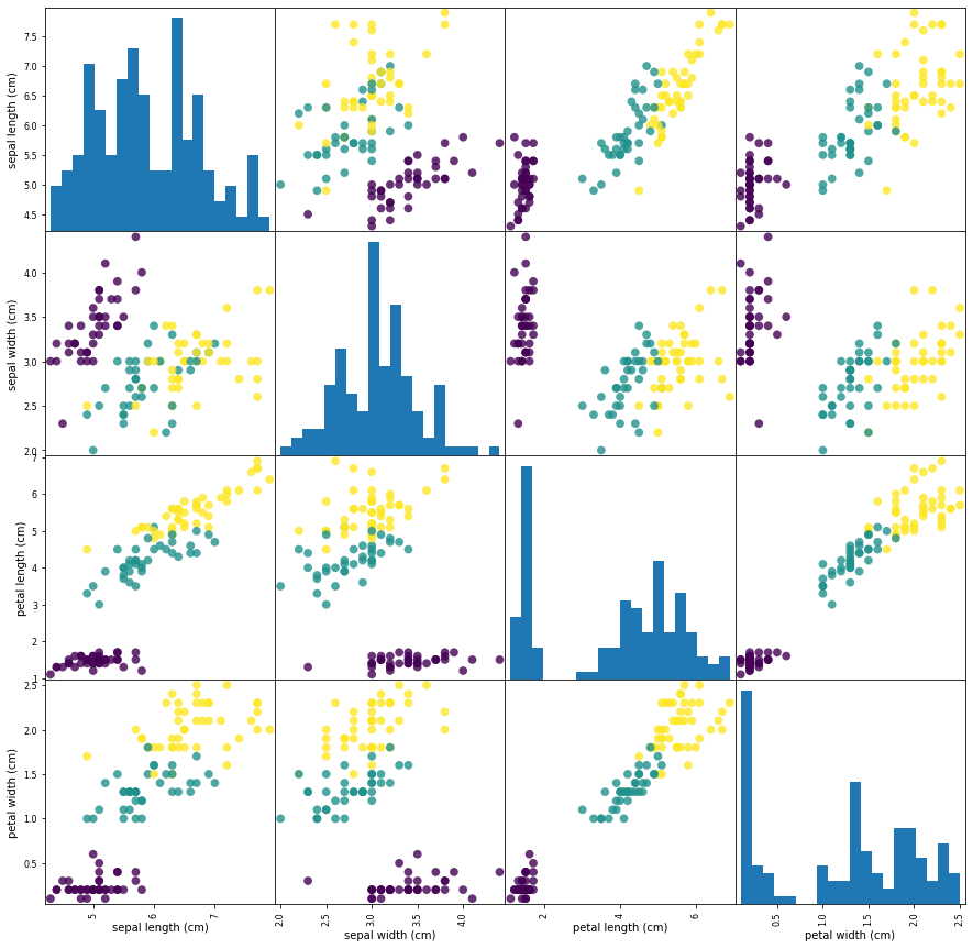
From the plots, we can see that the three classes seem to be relatively well separated using the sepal and petal measurements. This means that a machine learning model
will likely be able to learn to separate them.
First Model: k-Nearest Neighbors
The k-nearest neighbors (KNN) algorithm is a simple, easy-to-implement supervised machine learning algorithm that can be used to solve both classification and regression problems. The KNN algorithm assumes that similar things exist in close proximity. In other words, similar things are near to each other.
Building the k-nearest neighbors model only consists of storing the training set. To make a prediction for a new data point, the algorithm finds the point in the training set that is closest to the new point. Then it assigns the label of this training point to the new data point.
from sklearn.neighbors import KNeighborsClassifier
knn = KNeighborsClassifier(n_neighbors=1)
knn.fit(X_train, y_train)
Making Predictions: Imagine we found an iris in the wild with a sepal length of 5 cm, a sepal width of 2.9 cm, a petal length of 1 cm, and a petal width of 0.2 cm. What species of iris would this be?
X_new = np.array([[5, 2.9, 1, 0.2]])
print("X_new.shape: {}".format(X_new.shape))

prediction = knn.predict(X_new)
print("Prediction: {}".format(prediction))
print("Predicted target name: {}".format(
iris_dataset['target_names'][prediction]))
X_new.shape: (1, 4)
Prediction: [0]
Predicted target name: ['setosa']
Our model predicts that this new iris belongs to the class 0, meaning its species is setosa. But how do we know whether we can trust our model? We don’t know the correct species of this sample, which is the whole point of building the model.
Model Evaluation
This is where the test set that we created earlier comes in. This data was not used to build the model, but we do know what the correct species is for each iris in the test set. Therefore, we can make a prediction for each iris in the test data and compare it against its label (the known species). We can measure how well the model works by computing the accuracy, which is the fraction of flowers for which the right species was predicted:
y_pred = knn.predict(X_test)
print("Test set predictions:\n {}".format(y_pred))
print("Test set score: {:.2f}".format(np.mean(y_pred == y_test)))
print("Test set score: {:.2f}".format(knn.score(X_test, y_test)))
Test set predictions:
 [2 1 0 2 0 2 0 1 1 1 2 1 1 1 1 0 1 1 0 0 2 1 0 0 2 0 0 1 1 0]
Test set score: 0.98
Test set score: 0.98
Conclusion
For this model, the test set accuracy is about 0.98, which means we made the right prediction for 98% of the irises in the test set. This high level of accuracy means that ourmodel may be trustworthy enough to use!