Supervised Learning
Supervised learning is used whenever we want to predict a certain
outcome from a given input, and we have examples of input/output pairs. We build a
machine learning model from these input/output pairs, which comprise our training
set. Our goal is to make accurate predictions for new, never-before-seen data. Supervised
learning often requires human effort to build the training set, but afterward
automates and often speeds up an otherwise laborious or infeasible task.
Classification and Regression
There are two major types of supervised machine learning problems, called classification
and regression.
In classification, the goal is to predict a class label, which is a choice from a predefined
list of possibilities. You can think of binary classification as trying to answer a yes/no question.
Classifying emails as either spam or not spam is an example of a binary classification problem.
For regression tasks, the goal is to predict a continuous number, or a floating-point
number in programming terms (or real number in mathematical terms). Predicting a
person’s annual income from their education, their age, and where they live is an
example of a regression task. When predicting income, the predicted value is an
amount, and can be any number in a given range.
import sys
import pandas as pd
import matplotlib
import numpy as np
import scipy as sp
import sklearn
%matplotlib inline
import matplotlib.pyplot as plt
import seaborn as sns
from sklearn.datasets import load_breast_cancer
cancer = load_breast_cancer()
print("cancer.keys(): \n{}".format(cancer.keys()))
cancer.keys():
dict_keys(['data', 'target', 'frame', 'target_names', 'DESCR', 'feature_names', 'filename', 'data_module'])
Of these 569 data points, 212 are labeled as malignant and 357 as benign.
Model complexity and generalization: Analyzing the KNeighborsClassifier
We evaluate training and test set performance with different numbers of neighbors.
from sklearn.model_selection import train_test_split
from sklearn.neighbors import KNeighborsClassifier

X_train, X_test, y_train, y_test = train_test_split(cancer.data, cancer.target, stratify = cancer.target, random_state = 1000)

training_accuracy = []
test_accuracy = []
neighbors = range(1,11)

for n_neighbors in neighbors:
  kNN = KNeighborsClassifier(n_neighbors = n_neighbors)
  kNN.fit(X_train, y_train)
  training_accuracy.append(kNN.score(X_train, y_train))
  test_accuracy.append(kNN.score(X_test, y_test))

plt.plot(neighbors, training_accuracy, label = 'Training Accuracy')
plt.plot(neighbors, test_accuracy, label = 'Test Accuracy')
plt.ylabel('Accuracay')
plt.xlabel('n_neighbors')
plt.title('Comparison of training and test accuracy as a function of n_neighbors')
plt.legend()
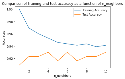
The plot shows the training and test set accuracy on the y-axis against the setting of n_neighbors on the x-axis. While real-world plots are rarely very smooth, we can still recognize some of the characteristics of overfitting and underfitting.
Considering a single nearest neighbor, the prediction on the training set is perfect. But when more neighbors are considered, the model becomes simpler and the training accuracy drops.
The test set accuracy for using a single neighbor is lower than when using more neighbors, indicating that using the single nearest neighbor leads to a model that is too complex. On the other hand, when considering 10 neighbors, the model is too simple and performance is even worse. The best performance is somewhere in the middle, using around 6 neighbors. Still, it is good to keep the scale of the plot in mind. The worst performance is around 88% accuracy, which might still be acceptable.
In principle, there are two important parameters to the KNeighbors classifier: the number of neighbors and how you measure distance between data points. In practice, using a small number of neighbors like three or five often works well, but you should certainly adjust this parameter.
One of the strengths of k-NN is that the model is very easy to understand, and often gives reasonable performance without a lot of adjustments. Using this algorithm is a good baseline method to try before considering more advanced techniques. Building the nearest neighbors model is usually very fast, but when your training set is very large (either in number of features or in number of samples) prediction can be slow.
One of the weaknesses of k-NN is that When using the k-NN algorithm, it’s important to preprocess your data. This approach often does not perform well on datasets with many features (hundreds or more), and it does particularly badly with datasets where most features are 0 most of the time (so-called sparse datasets).
Therefore, while the nearest k-neighbors algorithm is easy to understand, it is not often used in practice, due to prediction being slow and its inability to handle many features. The method we discuss next has neither of these drawbacks.
Linear Regression (aka ordinary least squares) Models
Linear models make a prediction using a linear function of the input features. Linear regression, or ordinary least squares (OLS), is the simplest and most classic linear method for regression. Linear regression finds the parameters that minimize the mean squared error between predictions and the true regression targets, y, on the training set. The mean squared error is the sum of the squared differencesnbetween the predictions and the true values. Linear regression has no parameters, which is a benefit, but it also has no way to control model complexity.
from sklearn.linear_model import LinearRegression
lin_reg = LinearRegression().fit(X_train, y_train)

print("Training set score: {:.2f}".format(lin_reg.score(X_train, y_train)))
print("Test set score: {:.2f}".format(lin_reg.score(X_test, y_test)))

print("lin_reg.coef_: {}".format(lin_reg.coef_))
print("lin_reg.intercept_: {}".format(lin_reg.intercept_))
Training set score: 0.78
Test set score: 0.75
lin_reg.coef_: [ 2.22681451e-01 -2.21641588e-03 -1.92758850e-02 -7.73163460e-04
 -1.76833636e-01  3.91229857e+00 -1.05795513e+00 -2.09565671e+00
 -5.30193958e-02  1.72639334e+00 -5.26019239e-01  1.44956000e-02
  3.19946586e-02  1.04006789e-03 -1.46111718e+01 -3.08559596e-01
  4.69096220e+00 -1.49353369e+01  6.83972184e-01 -2.11128905e+00
 -1.76597890e-01 -9.51329814e-03 -1.46851407e-03  1.10971442e-03
 -9.99186336e-01  1.15341813e-01 -7.62589750e-01  5.20310221e-01
 -9.37896191e-01 -3.69768514e+00]
lin_reg.intercept_: 2.8361789835644062
One of the most commonly used alternatives to standard linear regression is ridge regression.
Ridge Regression Models
Ridge regression is a method of estimating the coefficients of multiple-regression models in scenarios where linearly independent variables are highly correlated. It is also a linear model for regression, so the formula it uses to make predictions is the same one used for OLS. In ridge regression, though, the coefficients are chosen not only so that they predict well on the training data, but also to fit an additional constraint. We also want the magnitude of coefficients to be as small as possible. Intuitively, this means each feature should have as little effect on the outcome as possible (which translates to having a small slope), while still predicting well. This constraint is an example of what is called regularization. Regularization means explicitly restricting a model to avoid overfitting. The particular kind used by ridge regression is known as L2 regularization.
from sklearn.linear_model import Ridge

ridge = Ridge().fit(X_train, y_train)
print("Training set score: {:.2f}".format(ridge.score(X_train, y_train)))
print("Test set score: {:.2f}".format(ridge.score(X_test, y_test)))
Training set score: 0.74
Test set score: 0.74
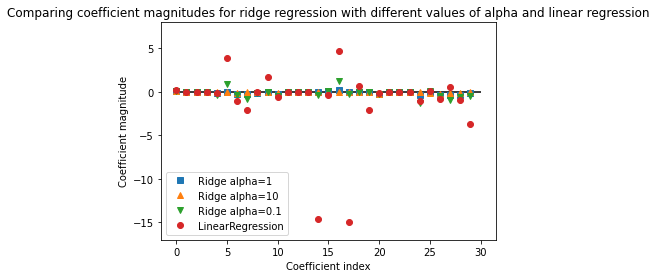
As you can see, the training set score of Ridge is lower than for LinearRegression, while the test set score is higher. This is consistent with our expectation. With linear regression, we were overfitting our data. Ridge is a more restricted model, so we are less likely to overfit.
Ridge is a more restricted model, so we are less likely to overfit. A less complex model means worse performance on the training set, but better generalization.
The Ridge model makes a trade-off between the simplicity of the model (near-zero coefficients) and its performance on the training set. How much importance the model places on simplicity versus training set performance can be specified by the user, using the alpha parameter.
Alpha (α) can be any real-valued number between zero and infinity; the larger the value, the more aggressive the penalization is.
Default alpha is alpha = 1.0. The optimum setting of alpha depends on the particular dataset we are using. Increasing alpha forces coefficients to move more toward zero, which decreases training set performance but might help generalization.
ridge10 = Ridge(alpha=10).fit(X_train, y_train)
print("Training set score: {:.2f}".format(ridge10.score(X_train, y_train)))
print("Test set score: {:.2f}".format(ridge10.score(X_test, y_test)))
Training set score: 0.72
Test set score: 0.72
Decreasing alpha allows the coefficients to be less restricted. For very small values of alpha, coefficients are barely restricted at all, and we end up with a model that resembles LinearRegression.
ridge01 = Ridge(alpha=0.1).fit(X_train, y_train)
print("Training set score: {:.2f}".format(ridge01.score(X_train, y_train)))
print("Test set score: {:.2f}".format(ridge01.score(X_test, y_test)))
Training set score: 0.76
Test set score: 0.75
plt.plot(ridge.coef_, 's', label="Ridge alpha=1")
plt.plot(ridge10.coef_, '^', label="Ridge alpha=10")
plt.plot(ridge01.coef_, 'v', label="Ridge alpha=0.1")
plt.plot(lin_reg.coef_, 'o', label="LinearRegression")
plt.xlabel("Coefficient index")
plt.ylabel("Coefficient magnitude")
plt.title("Comparing coefficient magnitudes for ridge regression with different values of alpha and linear regression")
plt.hlines(0, 0, len(lin_reg.coef_))
plt.ylim(-17, 8)
plt.legend()
In practice, ridge regression is usually the first choice between these two models. However, if you have a large amount of features and expect only a few of them to be important, Lasso might be a better choice.
Logistic Regression and Linear SVC
By default, both models apply an L2 regularization, in the same way that Ridge does for regression.
Also, for both LogisticRegression and LinearSVC, the trade-off parameter that determines the strength of the regularization is called C, and higher values of C correspond to less regularization (the inverse of the regularization strength). In other words, when you use a high value for the parameter C, Logistic Regression and LinearSVC try to fit the training set as best as possible, while with low values of the parameter C, the models put more emphasis on finding a coefficient vector (w) that is close to zero.
There is another interesting aspect of how the parameter C acts. Using low values of C will cause the algorithms to try to adjust to the “majority” of data points, while using a higher value of C stresses the importance that each individual data point be classified correctly.
By default, C = 1: