WG Ch5 Exercise Solutions
Rachel Lee
Last compiled: 2023-09-05 15:26:25.305239
I write and update the solutions everyday. Please let me know of any typos.
For Week 3: read WG chapters 1-3.
Chapter 3
3.2 Exercises
1. Run ggplot(data = mpg). What do you see?
library(tidyverse)
library(dplyr)
library(ggplot2)

ggplot(data = mpg)
This is an empty plot since no layers were added with geom function.
2. How many rows are in mtcars? How many columns?
nrow(mtcars)## [1] 32ncol(mtcars)## [1] 11There are 32 rows and 11 columns in mtcars.
3. What does the drv variable describe? Read the help
for ?mpg to
find out.
# ?mpg drv is the type of drive train, where f = front-wheel
drive, r = rear wheel drive, 4 = 4wd.
4. Make a scatterplot of hwy versus
cyl.
ggplot(mpg, aes(x = cyl, y = hwy)) +
  geom_point()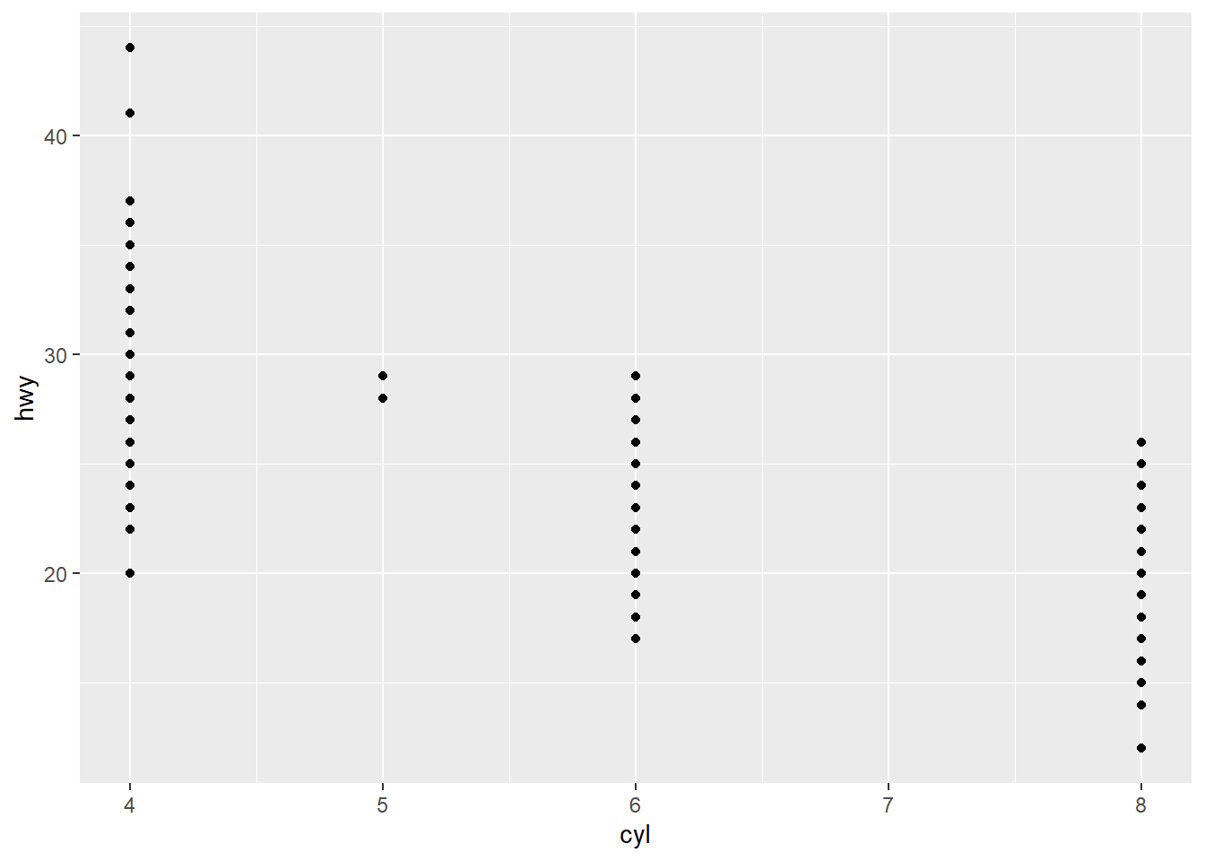
5. What happens if you make a scatterplot of class
versus drv?
Why is the plot not useful?
ggplot(mpg, aes(x = drv, y = class)) +
  geom_point()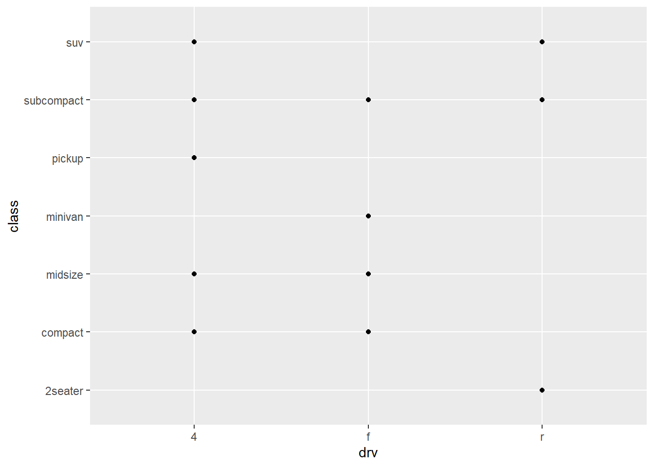
A scatter plot is not a useful here because both drv and
class are categorical variables. Scatterplots are commonly
used to visualize two continuous variables using visual marks mapped to
a two-dimensional Cartesian space. Hence, the scatterplot here shows the
limitation of managing two categorical variables. This is largely
because categorical variables are typically stored as a small number of
values. Within the mpg dataset, we can see that
class variables holds 7 types of cars, and cyl
holds 4 types of cylinders. Therefore, there will only be 21 points
mapped on the scatterplot.
mpg %>% distinct(class) # or unique(mpg$class)## # A tibble: 7 × 1
## class
## <chr>
## 1 compact
## 2 midsize
## 3 suv
## 4 2seater
## 5 minivan
## 6 pickup
## 7 subcompactmpg %>% distinct(cyl) # or unique(mpg$cyl)## # A tibble: 4 × 1
## cyl
## <int>
## 1 4
## 2 6
## 3 8
## 4 5
3.3 Exercises
1. What’s gone wrong with this code? Why are the points not blue?
ggplot(data = mpg) +
  geom_point(mapping = aes(x = displ, y = hwy, color = "blue"))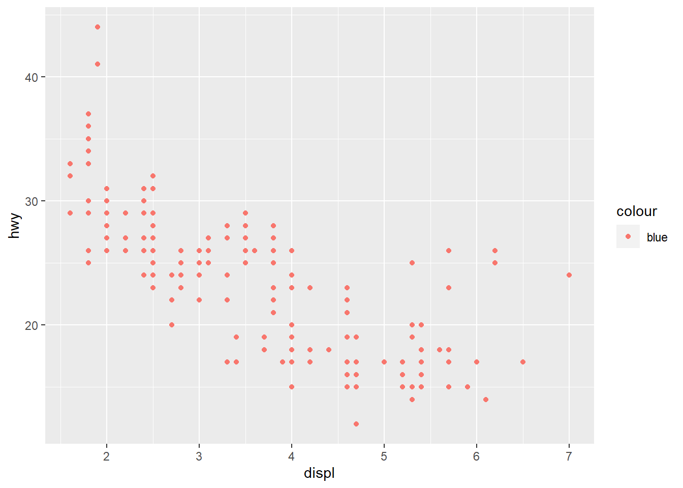
The color argument is defined as part of the
mapping. Therefore, it is being argued as an aesthetic.
This can be corrected as below:
ggplot(data = mpg) +
  geom_point(mapping = aes(x = displ, y = hwy), color = "blue")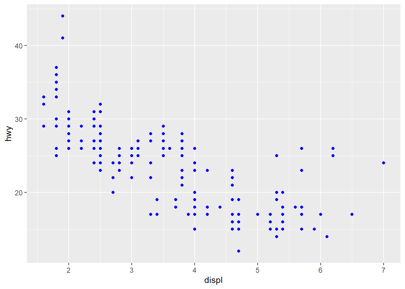
Or,
ggplot(data = mpg, aes(x = displ, y = hwy)) +
  geom_point(colour = "blue")
2. Which variables in mpg are categorical? Which
variables are continuous? (Hint: type ?mpg to read the
documentation for the dataset). How can you see this information when
you run mpg?
head(mpg, 10) # or glimpse(mpg)## # A tibble: 10 × 11
## manufacturer model displ year cyl trans drv cty hwy fl class
## <chr> <chr> <dbl> <int> <int> <chr> <chr> <int> <int> <chr> <chr>
## 1 audi a4 1.8 1999 4 auto… f 18 29 p comp…
## 2 audi a4 1.8 1999 4 manu… f 21 29 p comp…
## 3 audi a4 2 2008 4 manu… f 20 31 p comp…
## 4 audi a4 2 2008 4 auto… f 21 30 p comp…
## 5 audi a4 2.8 1999 6 auto… f 16 26 p comp…
## 6 audi a4 2.8 1999 6 manu… f 18 26 p comp…
## 7 audi a4 3.1 2008 6 auto… f 18 27 p comp…
## 8 audi a4 quattro 1.8 1999 4 manu… 4 18 26 p comp…
## 9 audi a4 quattro 1.8 1999 4 auto… 4 16 25 p comp…
## 10 audi a4 quattro 2 2008 4 manu… 4 20 28 p comp…My initial screening is that Variables with <chr>
are categorical, those with <dbl> and
<int> are continuous. If you take a closer look at
the dataset, cyl, disp can be treated as
categorical since there are categories of values the cars are stored
under. year, city, and
hwydiscrete variables, but we can decide to treat it as
continuous variables.
3. Map a continuous variable to color,
size, and shape. How do these aesthetics
behave differently for categorical vs. continuous variables?
ggplot(mpg, aes(x = cty, y = hwy, color = drv)) +
  geom_point() +
  labs(title = "mpg dataset: hwy vs. cty",
       caption = "mpg dataset",
       x = "Highway miles per gallon",
       y = "city miles per gallon",
       color = "Type of drive train")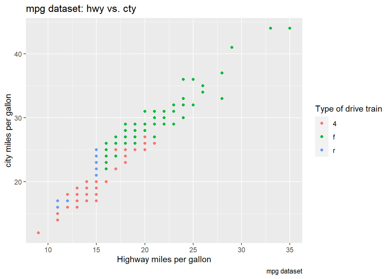
It’s intuitive that cty and hwy will show a
positive linear relationship. The color mapping is set to
drv, which is a categorical variable.
ggplot(mpg, aes(x = cty, y = hwy, color = cyl)) +
geom_point() +
labs(title = "mpg dataset: hwy vs. cty",
caption = "mpg dataset",
x = "Highway miles per gallon",
y = "city miles per gallon",
color = "Number of cylinders")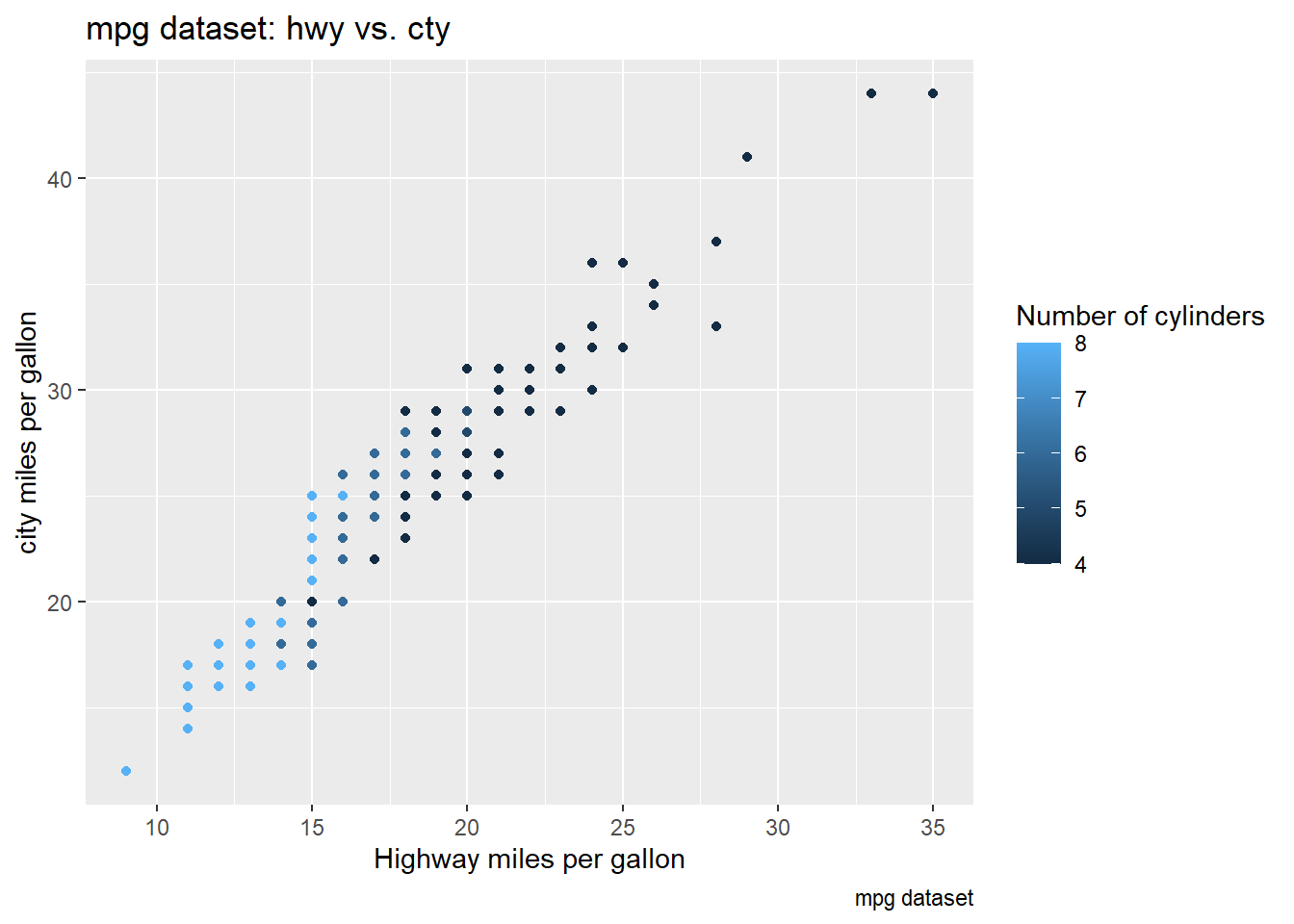 Now we set our
 color mapping to cyl, a
continuous variable. The difference between mapping color
to a categorical vs continuous variables is the legend. For categorical
variables, distinct categories are created as the legend, while gradient
scale is created for continuous variables.
Now, let’s take a look at the difference of categorical and
continuous variables being mapped to size:
ggplot(mpg, aes(x = cty, y = hwy, size = drv)) +
  geom_point() +
  labs(title = "mpg dataset: hwy vs. cty",
       caption = "mpg dataset",
       x = "Highway miles per gallon",
       y = "city miles per gallon",
       size = "Type of drive train")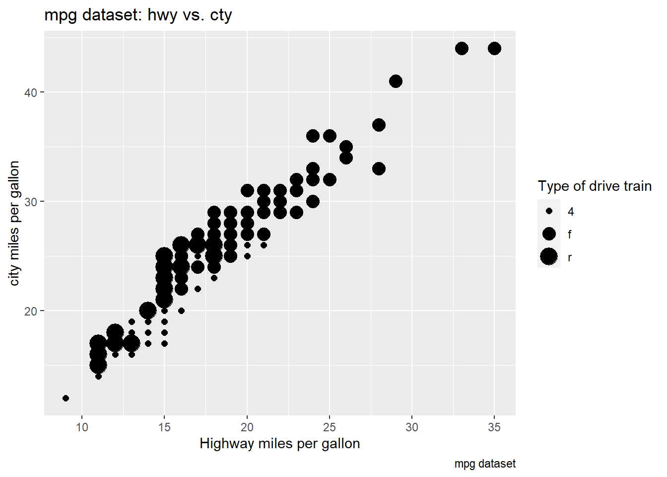
ggplot(mpg, aes(x = cty, y = hwy, size = cyl)) +
  geom_point() +
  labs(title = "mpg dataset: hwy vs. cty",
       caption = "mpg dataset",
       x = "Highway miles per gallon",
       y = "city miles per gallon",
       size = "Number of cylinders")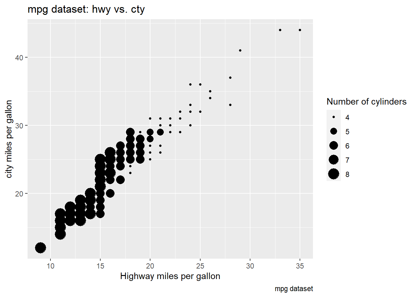
When mapped to size, the sizes of the points vary continuously as a function of their size.
Now, let’s assign the different variables types to
shape.
ggplot(mpg, aes(x = cty, y = hwy, shape = drv)) +
geom_point() +
labs(title = "mpg dataset: hwy vs. cty",
caption = "mpg dataset",
x = "Highway miles per gallon",
y = "city miles per gallon",
shape = "Type of drive train")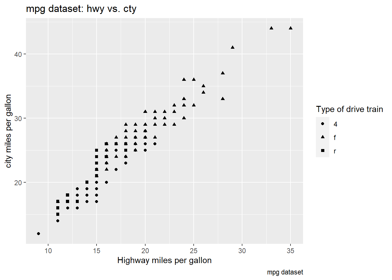 When the categorical variable is mapped to
 shape, three
types of drive train are assigned to different pointer shapes, and are
mapped on the graph accordingly. Intuitively, we will not be able to map
a continuous variable to shape. If you do, you will get the following
error message from R:
Error: A continuous variable can not be mapped to shape Runrlang::last_error()to see where the error occurred.
4. What happens if you map the same variable to multiple aesthetics?
ggplot(mpg, aes(x = cty, y = hwy, size = cty, color = hwy, shape = drv)) +
geom_point() +
labs(title = "mpg dataset: hwy vs. cty",
caption = "mpg dataset",
x = "Highway miles per gallon",
y = "city miles per gallon",
size = "city miles per gallon",
color = "Highway miles per gallon",
shape = "Type of drive train")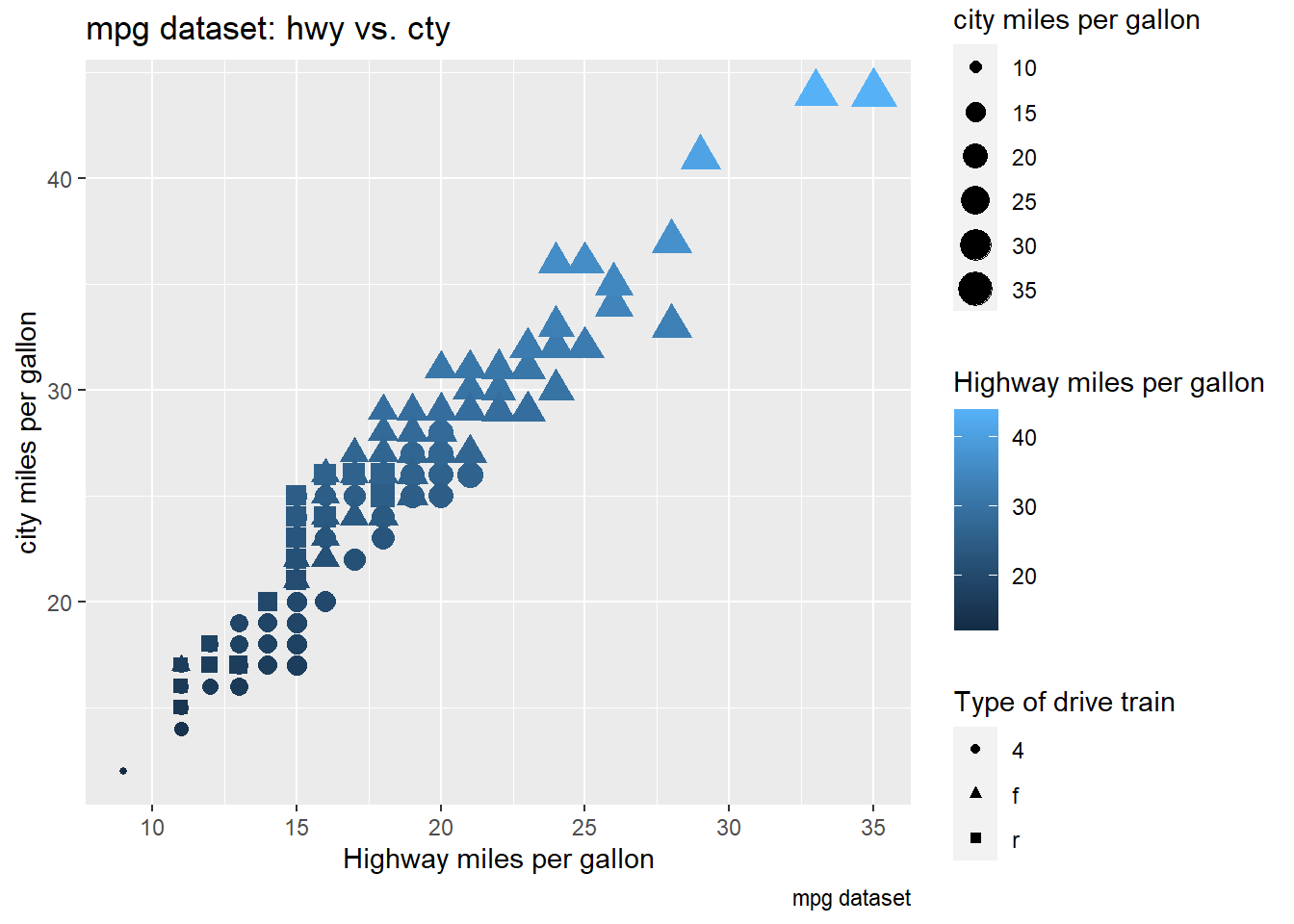 In the plot above, I mapped
 cty to both x-axis and size,
and hwy to y-axis and color. The R runs and produces the
messy graph due to redundant information. This is not advised - mapping
a single varialbe to multiple aesthetics is a bad practice and should be
avoided.
5. What does the stroke aesthetic do? What shapes does
it work with? (Hint: use ?geom_point)
# ?geom_point
ggplot(mpg, aes(x = displ, y = cty)) +
  geom_point(shape = 23, color = "#CC79A7", fill = "#F0E442", size = 3, stroke = 2)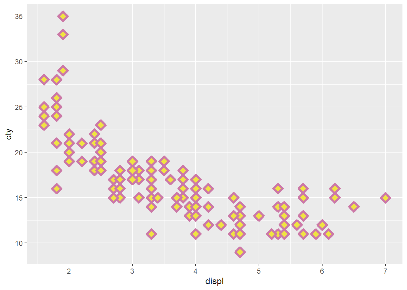
The stroke aesthetically modifies the width of the
border for shapes. It works with shapes numbering 21 through 25, which
are shapes that take the fill command with a specific
color.
6. What happens if you map an aesthetic to something other than a
variable name, like aes(colour = displ < 5)? Note,
you’ll also need to specify x and y.
ggplot(mpg, aes(x = cty, y = hwy, color = displ < 5)) +
  geom_point()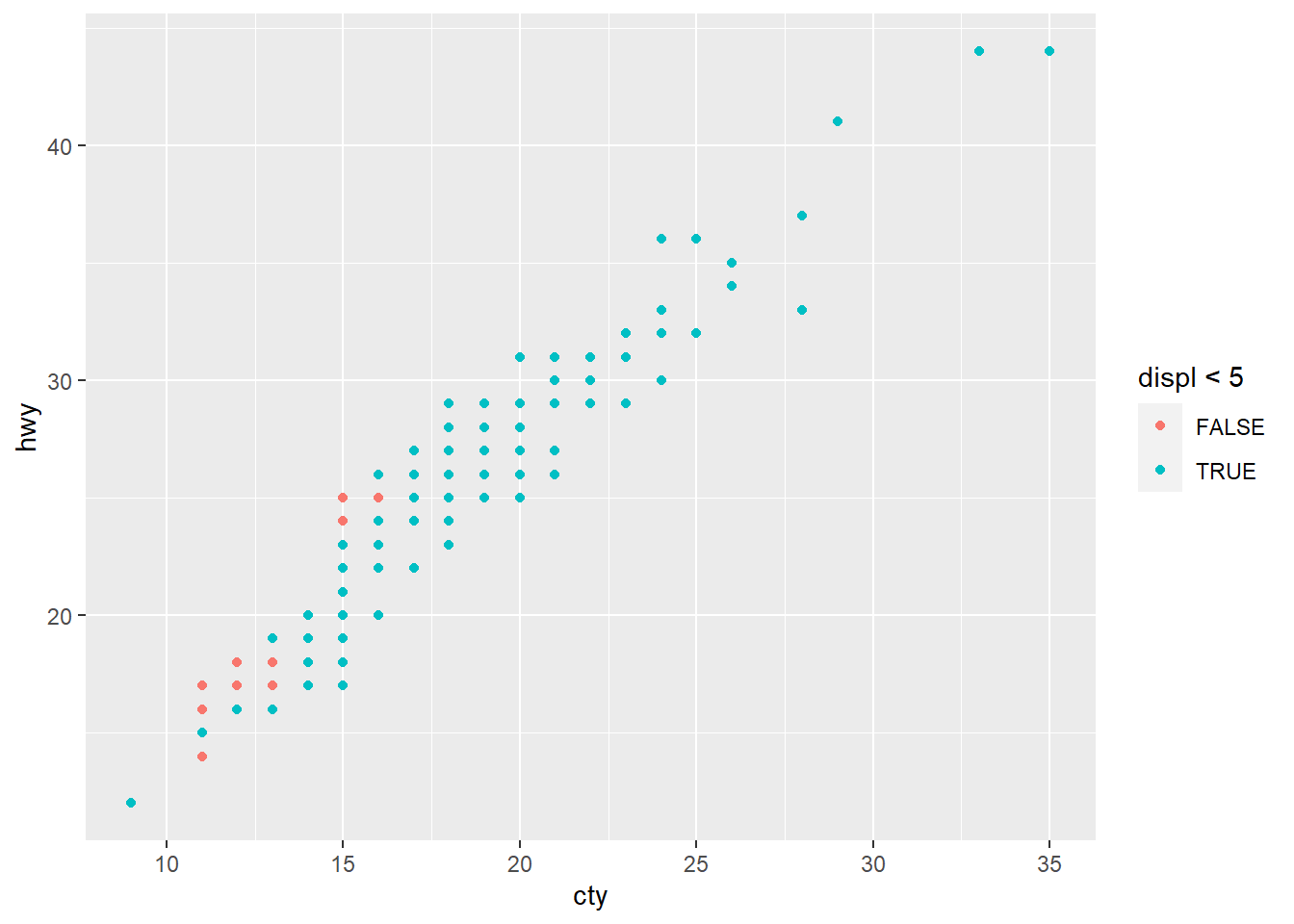
You are able to specify equations as well as expressions for
aesthetic mappings. In this case, displ < 5 will return
either TRUE or FALSE.
3.5 Exercises
1. What happens if you facet on a continuous variable?
ggplot(mpg, aes(x = displ, y = hwy)) +
  geom_point() +
  facet_wrap(. ~ hwy)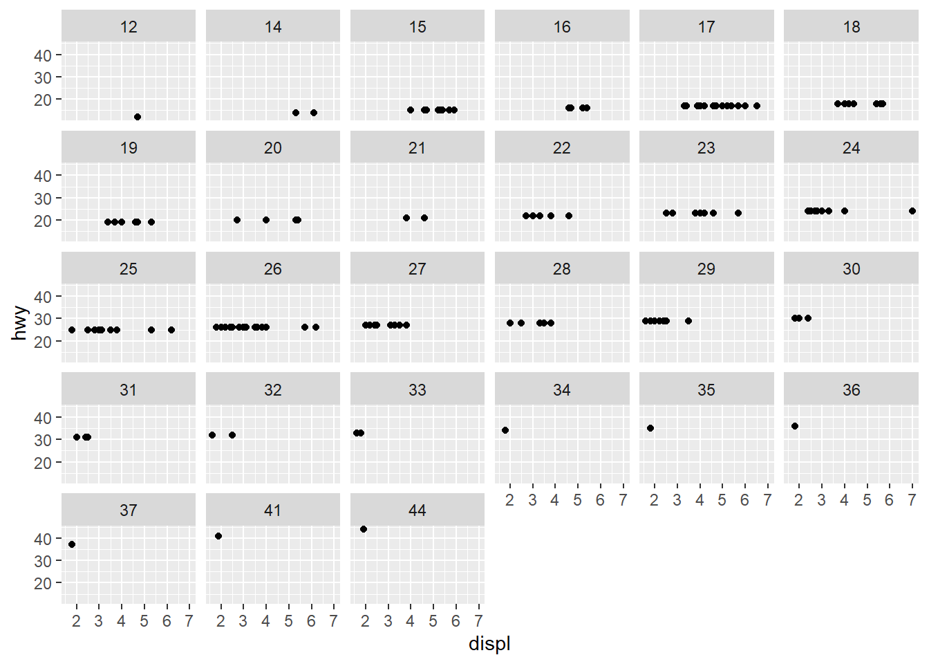
ggplot(mpg, aes(x = displ, y = hwy)) +
  geom_point() +
  facet_grid(. ~ hwy)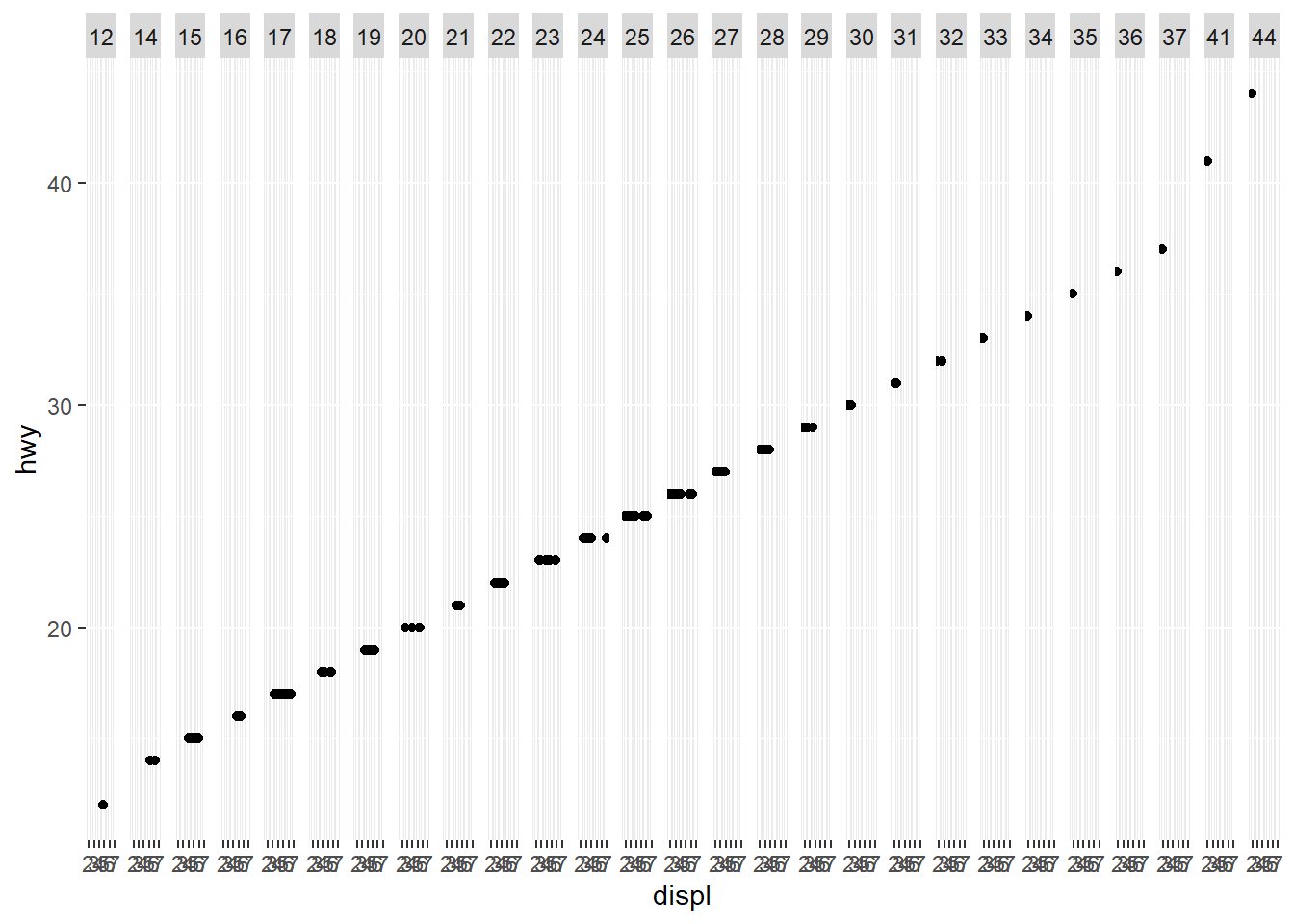
The primary use of facets is to add another categorical variable to
your plot. The variable that you pass to facet_wrap()
should be discrete. If you pass continuous variable, then it is
converted to a categorical variable, and the plot will contain a facet
for each distinct value.
2. What do the empty cells in plot with
facet_grid(drv ~ cyl) mean? How do they relate to this
plot?
ggplot(data = mpg) +
  geom_point(mapping = aes(x = drv, y = cyl))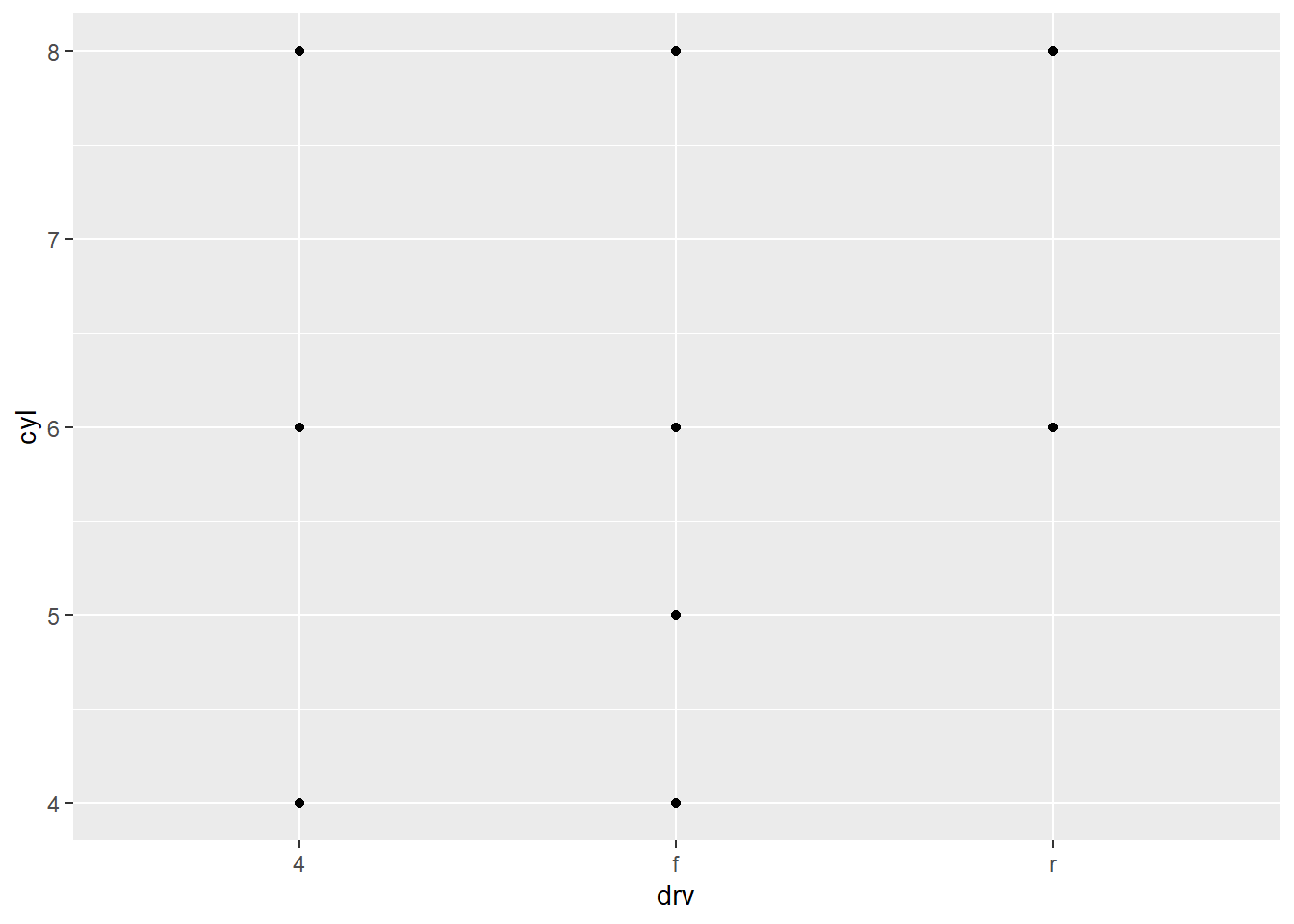
ggplot(data = mpg) +
  geom_point(mapping = aes(x = cty, y = hwy)) +
  facet_grid(drv ~ cyl)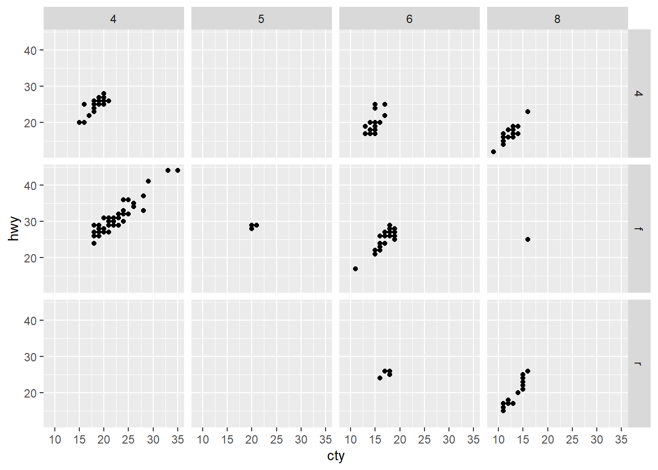
The scatterplot of drv and cyl shows empty
plots, and the empty cells matches where combinations of the two
variables have no observations.
3. What plots does the following code make? What does .
do?
ggplot(data = mpg) +
  geom_point(mapping = aes(x = displ, y = hwy)) +
  facet_grid(drv ~ .)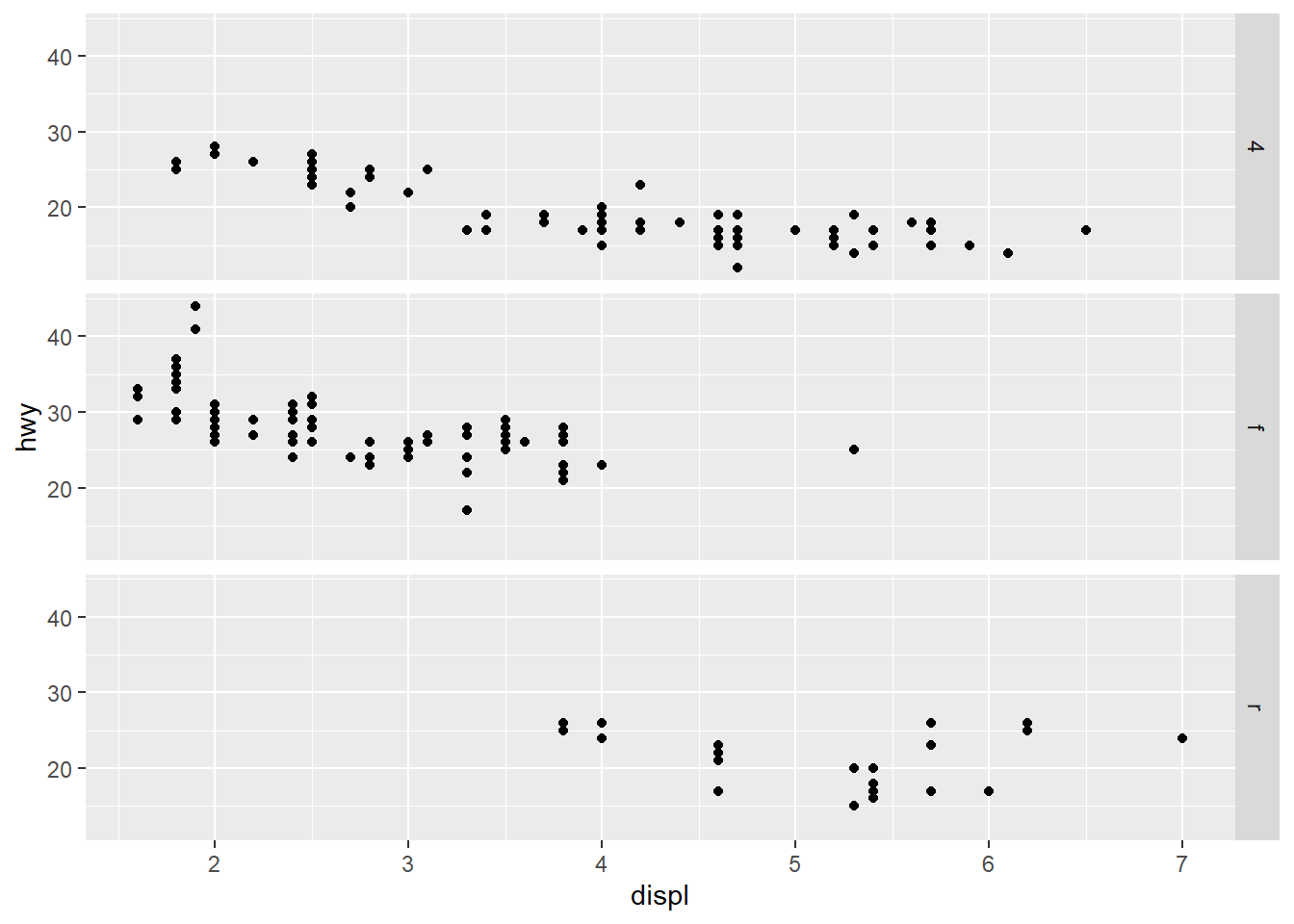
ggplot(data = mpg) +
  geom_point(mapping = aes(x = displ, y = hwy)) +
  facet_grid(. ~ cyl)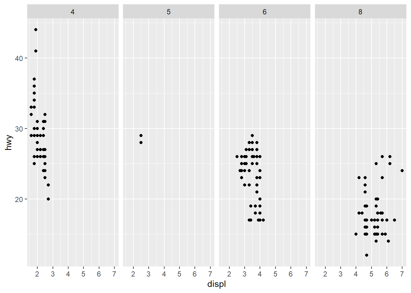
Everything on the left of the ~ will split according to
rows, and everything on the right will split to columns. The
. on the right hand side of the formula
(. ~ cyl) fixes the cyl variable on the
x-axis. If you want to flip the facets, this can be done as
cyl ~ ..
4. Take the first faceted plot in this section:
ggplot(data = mpg) +
geom_point(mapping = aes(x = displ, y = hwy)) +
facet_wrap(~ class, nrow = 2)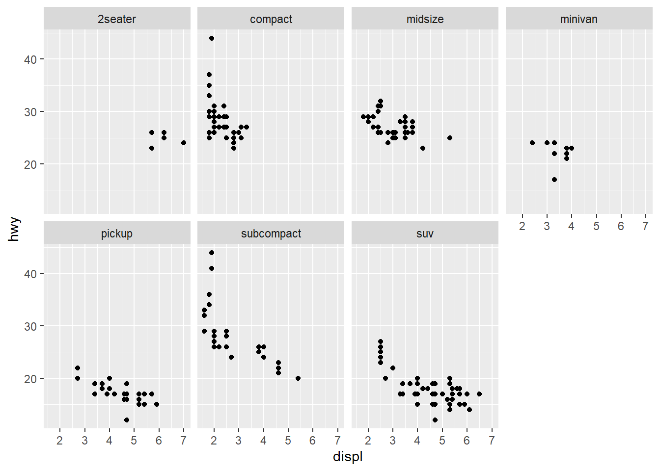 What are the advantages to using faceting instead of the color
aesthetic? What are the disadvantages? How might the balance change if
you had a larger dataset?
What are the advantages to using faceting instead of the color
aesthetic? What are the disadvantages? How might the balance change if
you had a larger dataset?
Let’s take the provided code, but add the color aesthetic instead of using faceting:
ggplot(data = mpg) +
geom_point(mapping = aes(x = displ, y = hwy, color = trans))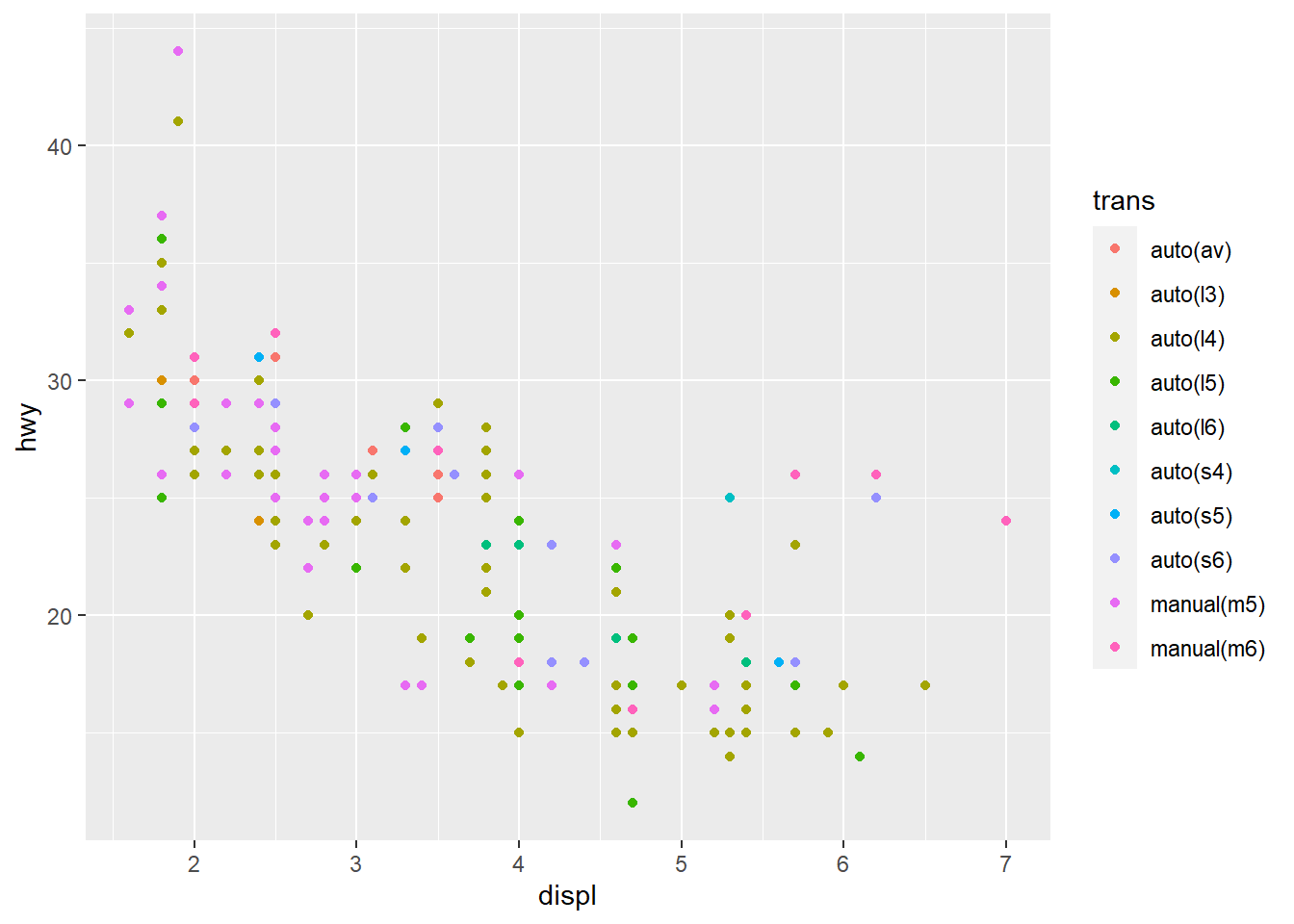 The advantage of adding color mapping is that we are able to add more
information to the graph. For instance, we are now able to distinguish
between the different types of transmission between engine displacement
and highway miles per hour variables across type of cars. Note that
using the color aesthetic can work against if there are many categories.
In this case, readers may have a hard time differentiating the colors
between manual(m5) and manual(m6).
The advantage of adding color mapping is that we are able to add more
information to the graph. For instance, we are now able to distinguish
between the different types of transmission between engine displacement
and highway miles per hour variables across type of cars. Note that
using the color aesthetic can work against if there are many categories.
In this case, readers may have a hard time differentiating the colors
between manual(m5) and manual(m6).
The disadvantage of using faceting instead of the color aesthetic is the difficulty of comparing the observations between categories plotted across different plots. It is much easier to interpret the graph if the observations are plotted on the same x- and y-scales.
5. Read ?facet_wrap. What does nrow do?
What does ncol do? What other options control the layout of
the individual panels? Why doesn’t facet_grid() have
nrow and ncol arguments?
# ?facet_wrap
# ?facet_grid
nrow and ncol refers to the number of rows
and columns used when laying out the facets. These arguments are needed
given that facet_wrap() only takes one variable to create
facets. The arguments does not exist for facet_grid()
because the function determines the number of rows and columns from the
unique values of the specified variables.
6. When using facet_grid() you should usually put the
variable with more unique levels in the columns. Why?
The simple reason is that there is more space for columns if the plots are laid out horizontally.
3.6 Exercises
1. What geom would you use to draw a line chart? A boxplot? A histogram? An area chart?
geom_line(): line chartgeom_boxplot(): boxplotgeom_histogram(): histogramgeom_area(): area chart
2. Run this code in your head and predict what the output will look like. Then, run the code in R and check your predictions.
geom_point() will create a scatterplot with
displ on the x-axis, hwy on the y-axis,
drv grouped and colored. geom_smooth() will
create a smooth line, and se = FALSE will suppress standard
errors.
ggplot(data = mpg, mapping = aes(x = displ, y = hwy, color = drv)) +
  geom_point() +
  geom_smooth(se = FALSE)
3. What does show.legend = FALSE do? What happens if
you remove it? Why do you think I used it earlier in the chapter?
The code below is from this chapter where the authors have
show.legend = FALSE.
ggplot(data = mpg) +
  geom_smooth(
    mapping = aes(x = displ, y = hwy, colour = drv),
    show.legend = FALSE
  )
Here is the same code with show.legend = TRUE:
ggplot(data = mpg) +
  geom_smooth(
    mapping = aes(x = displ, y = hwy, colour = drv),
    show.legend = TRUE
  )
Adding the legend would be beneficial if the authors decided to use a
single graph. However, with three graphs adjacent to each other, adding
a legend to only the last graph may confuse readers, as well as offset
the plot sizes. Moreover, the authors intention of using the three
graphs altogether was to show the difference adding extra
group or color mappings to aesthetics.
Therefore, legend was not necessary.
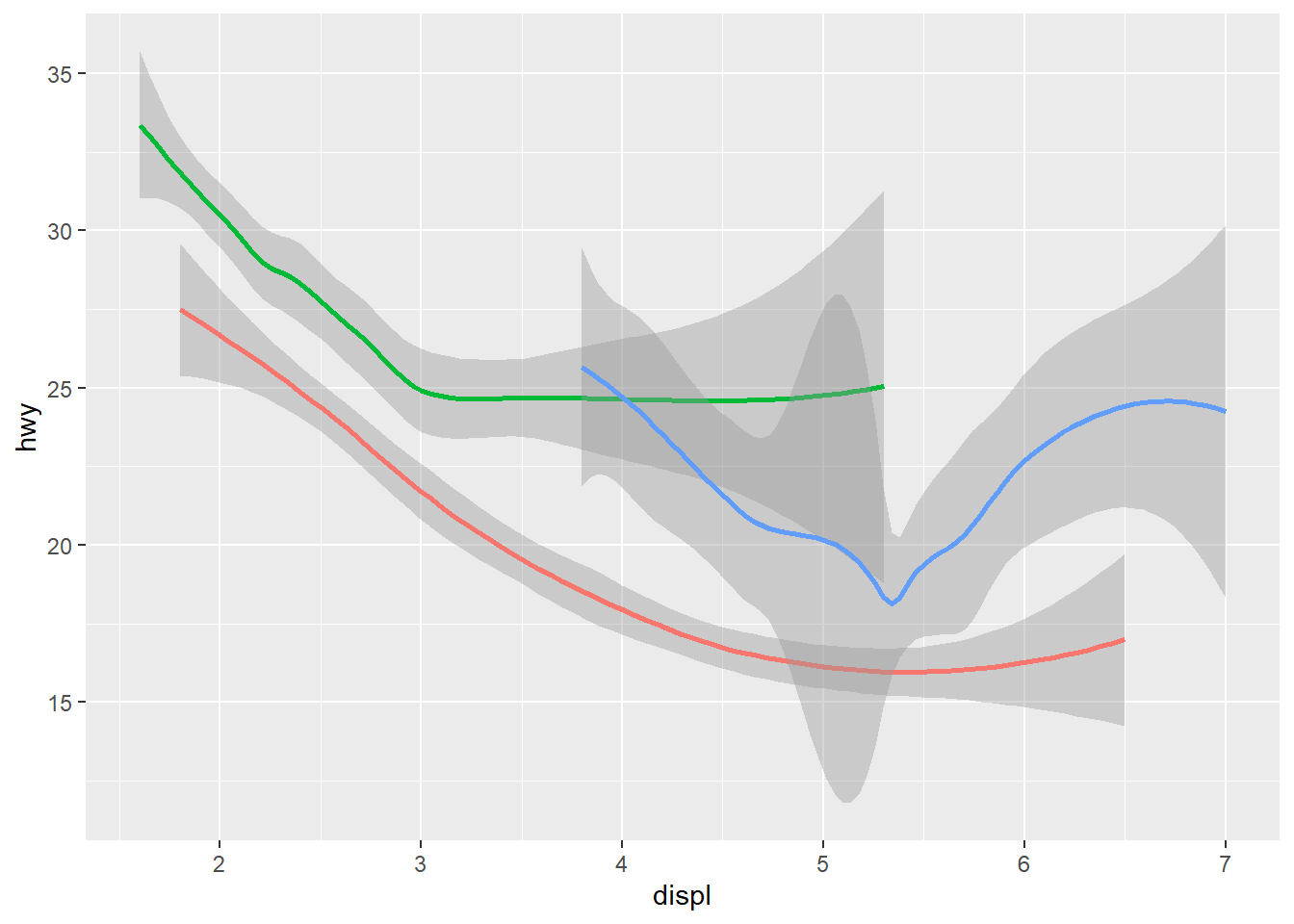
4. What does the se argument to
geom_smooth() do?
ggplot(data = mpg, mapping = aes(x = displ, y = hwy)) +
  geom_point(mapping = aes(color = class)) +
  geom_smooth(data = filter(mpg, class == "subcompact"), se = FALSE)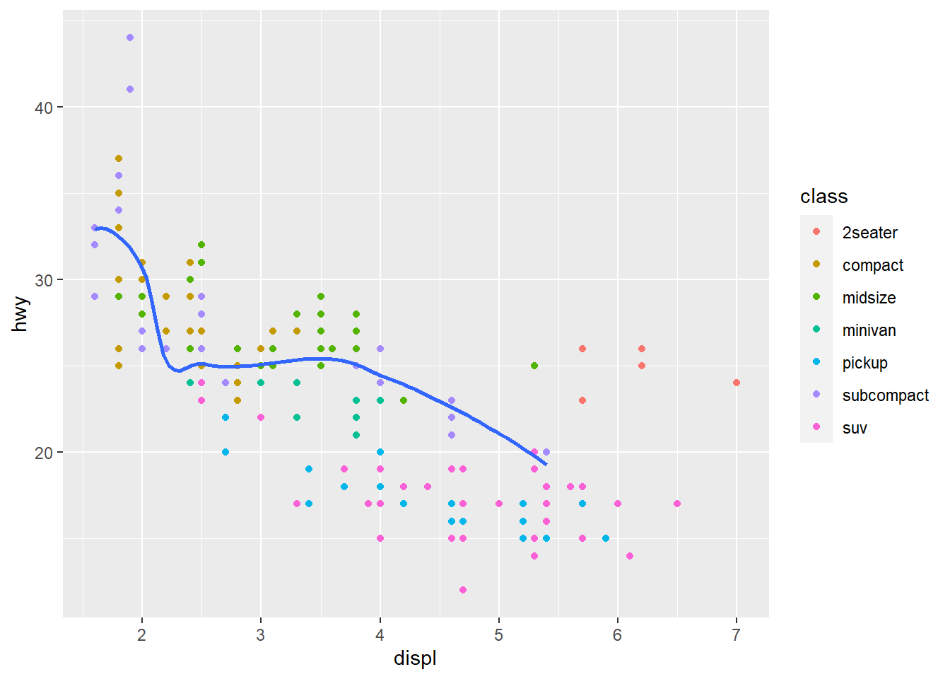
ggplot(data = mpg, mapping = aes(x = displ, y = hwy)) +
  geom_point(mapping = aes(color = class)) +
  geom_smooth(data = filter(mpg, class == "subcompact"), se = TRUE)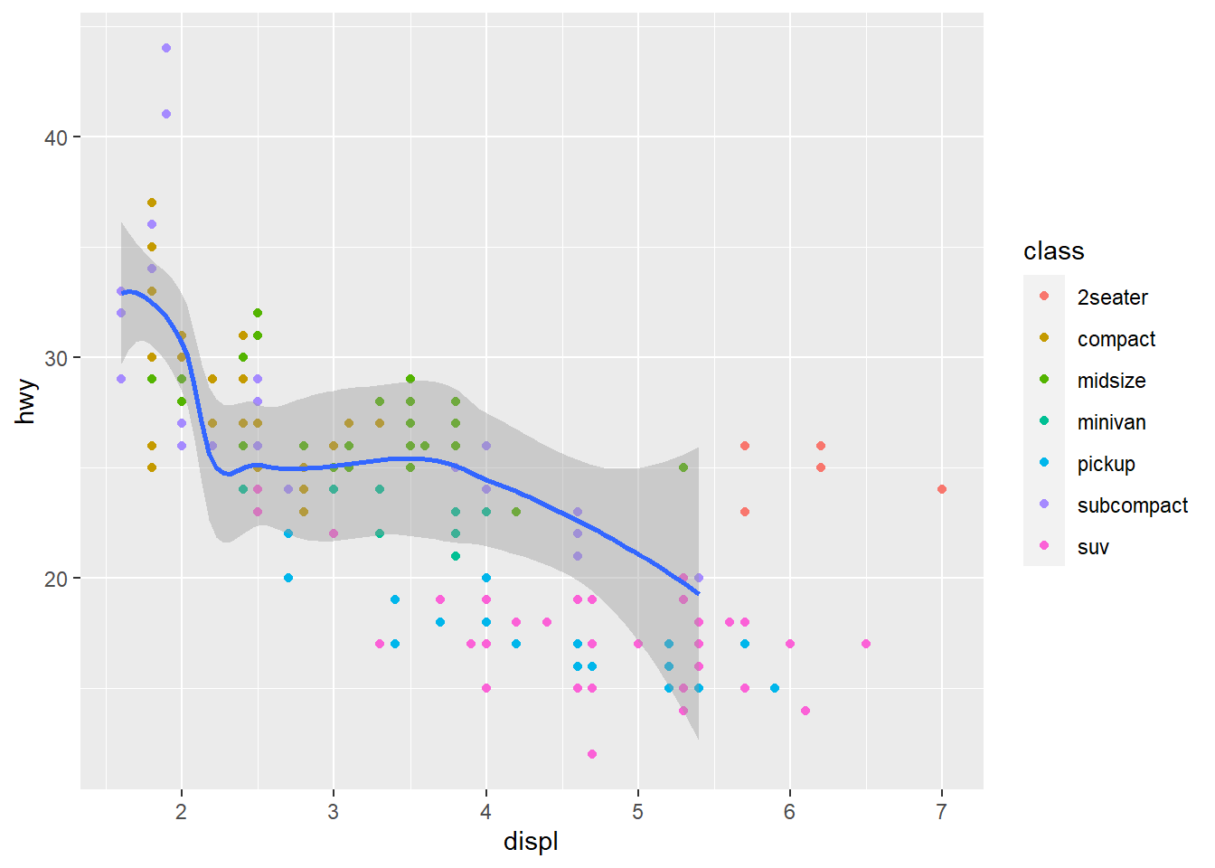
As it can be seen from the two graphs, the se argument
adds the standard error bands to the lines.
5. Will these two graphs look different? Why/why not?
ggplot(data = mpg, mapping = aes(x = displ, y = hwy)) +
  geom_point() +
  geom_smooth()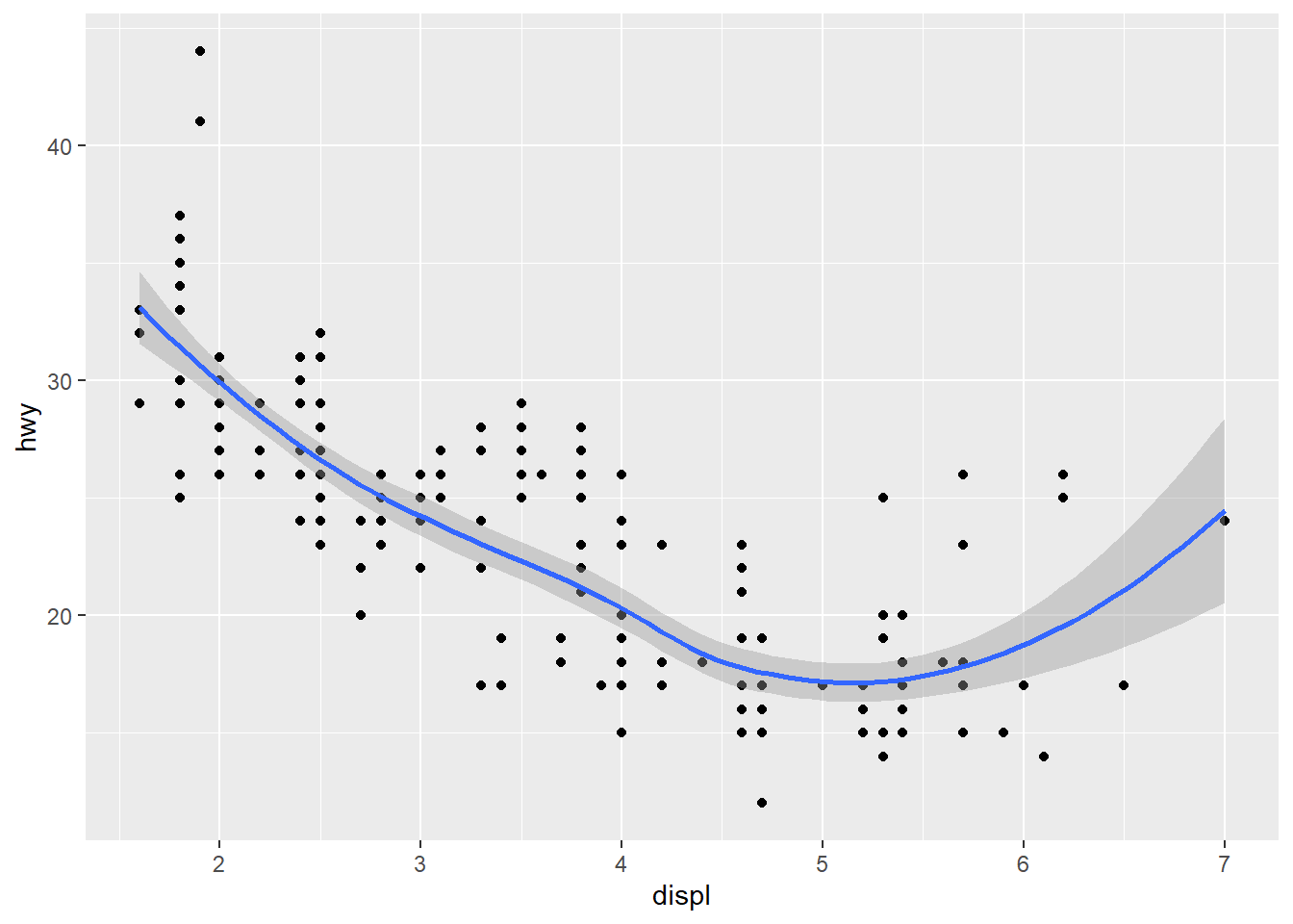
ggplot() +
  geom_point(data = mpg, mapping = aes(x = displ, y = hwy)) +
  geom_smooth(data = mpg, mapping = aes(x = displ, y = hwy))
The first set of code has the mapping:
aes(x = displ, y = hwy), which is passed down to
geom_point() and geom_smooth(). For the second
set of code, it still uses the same mapping for both
geom_point() and geom_smooth() through
specification. Therefore, the two graphs will look identical.
6. Recreate the R code necessary to generate the following graphs.
ggplot(mpg, aes(x = displ, y = hwy)) +
  geom_point() +
  geom_smooth(se = FALSE)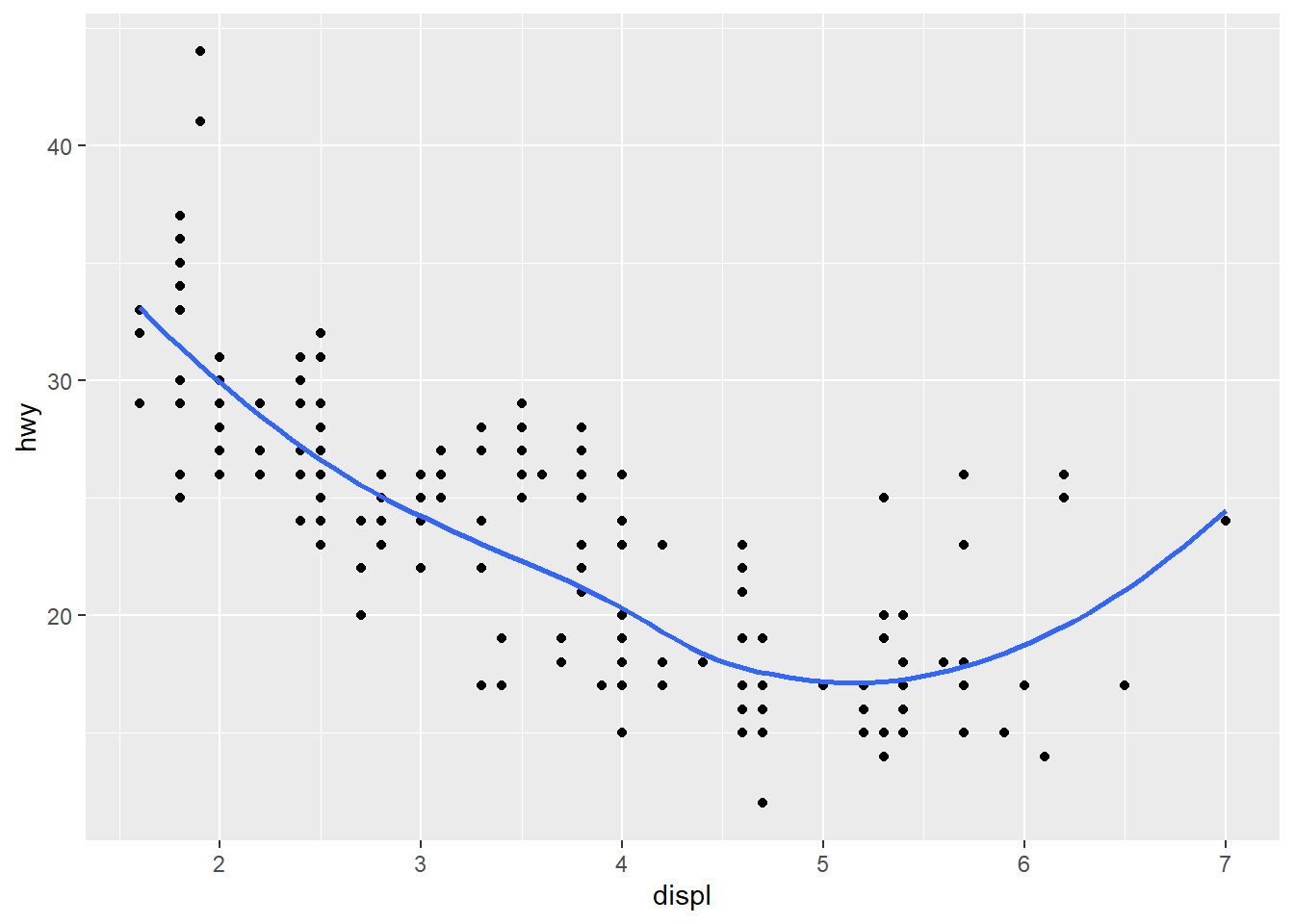
ggplot(mpg, aes(x = displ, y = hwy)) +
  geom_point() +
  geom_smooth(aes(group=drv), se = FALSE)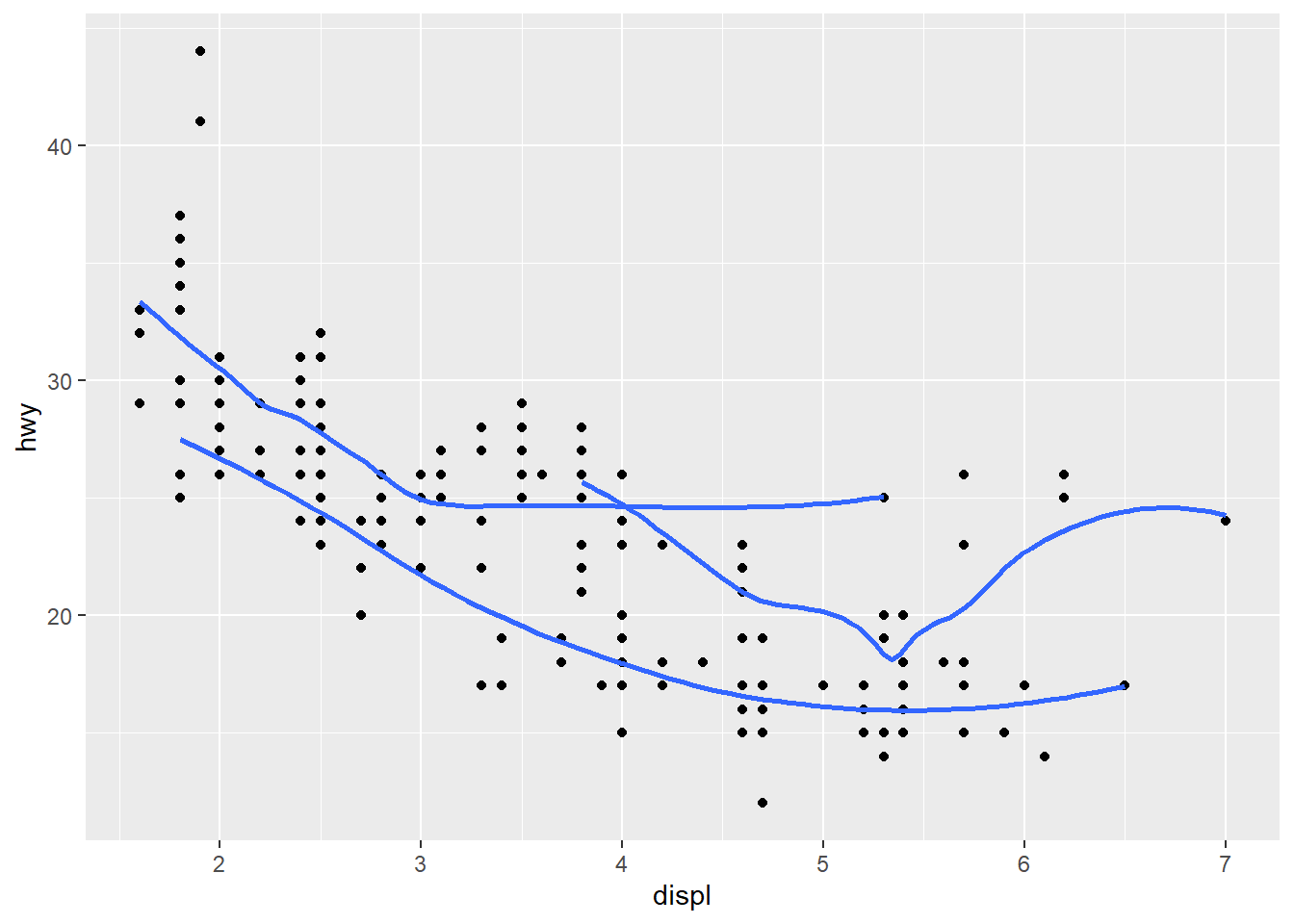
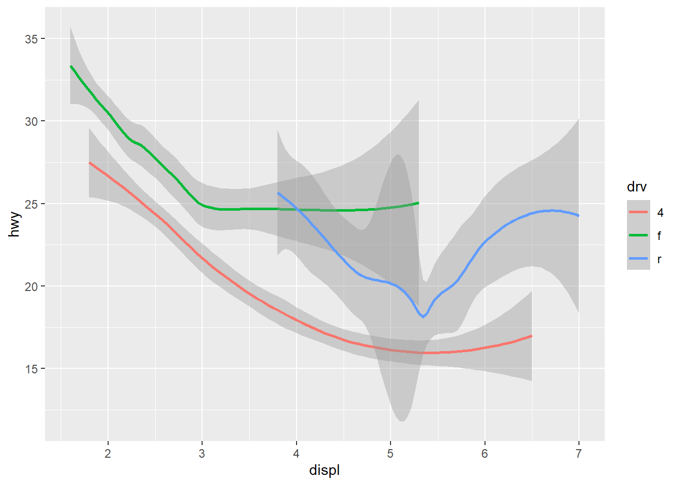
ggplot(mpg, aes(x = displ, y = hwy, color = drv)) +
  geom_point() +
  geom_smooth(se = FALSE)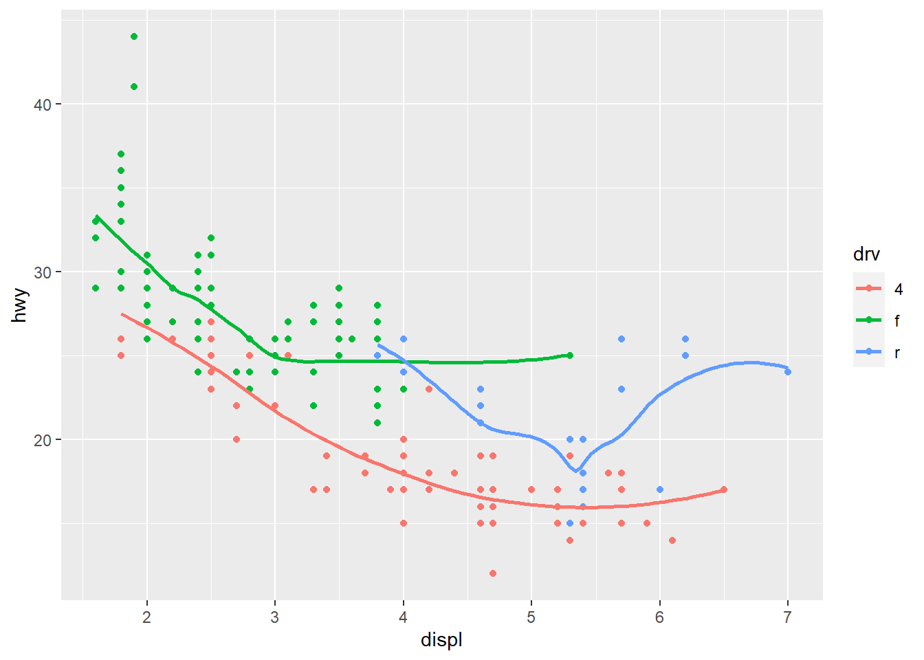
ggplot(mpg, aes(x = displ, y = hwy)) +
  geom_point(aes(color = drv)) +
  geom_smooth(se = FALSE)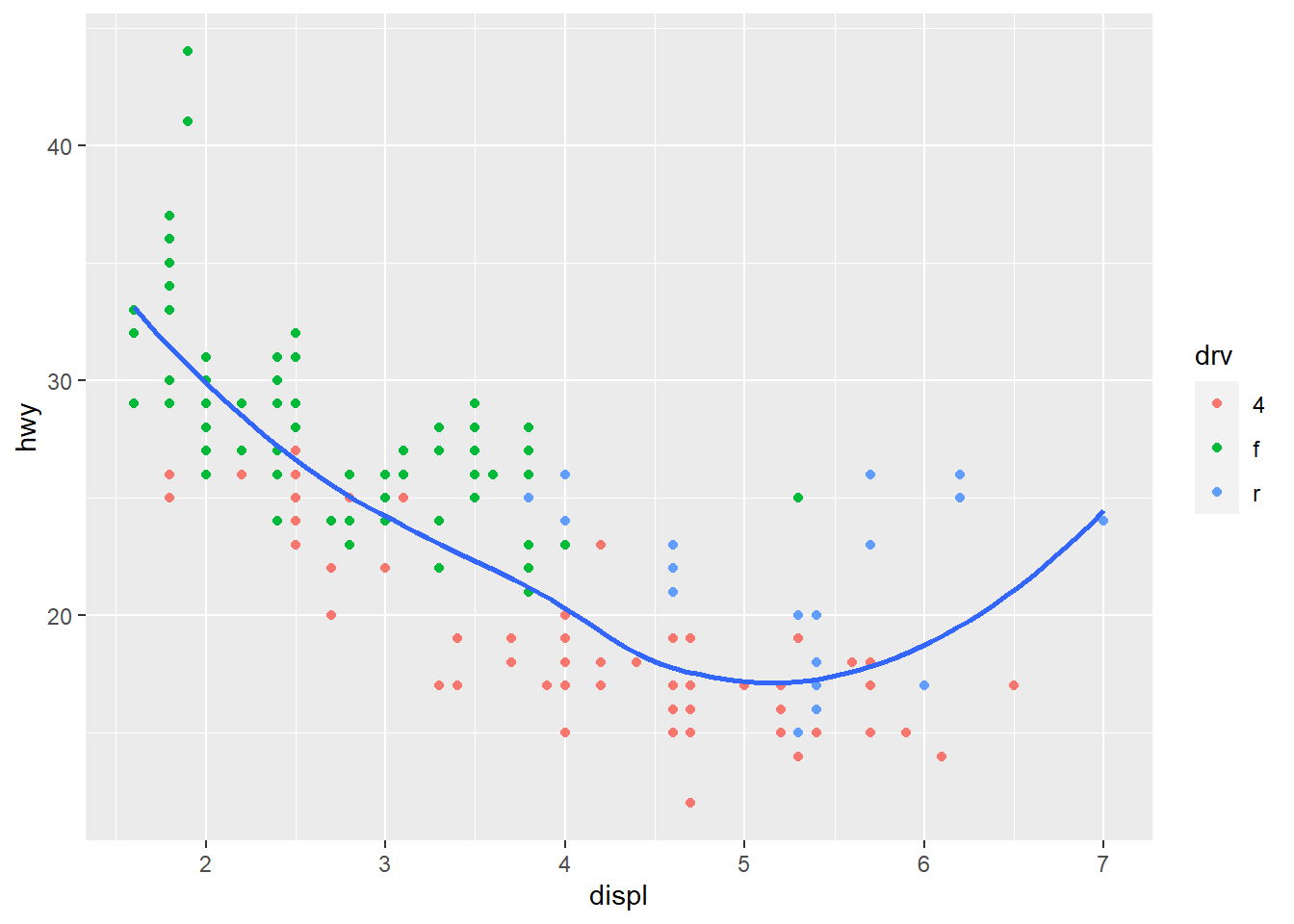
ggplot(mpg, aes(x = displ, y = hwy)) +
  geom_point(aes(color = drv)) +
  geom_smooth(aes(linetype = drv), se = FALSE)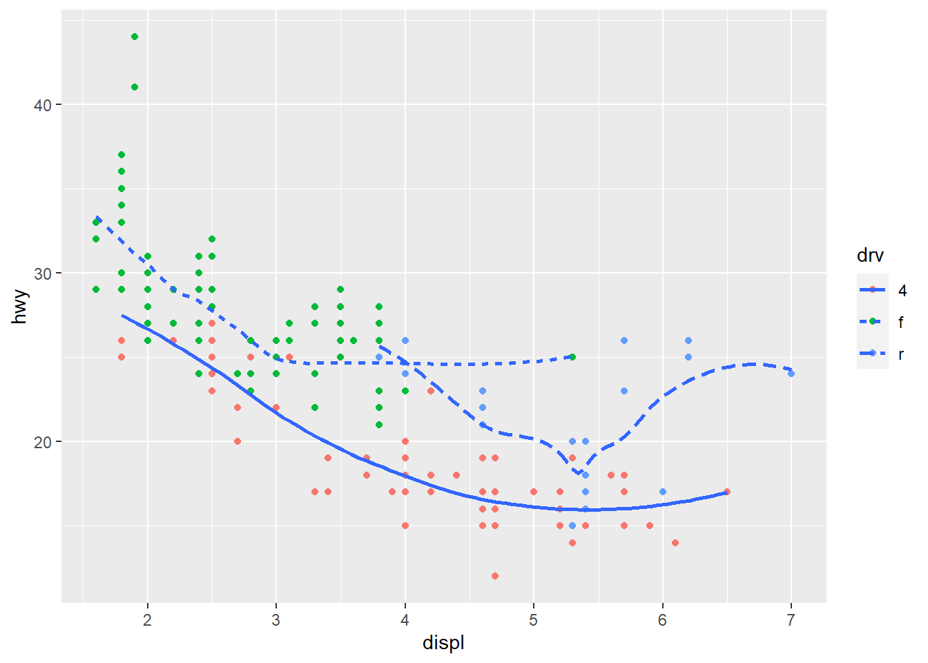
ggplot(mpg, aes(x = displ, y = hwy)) +
  geom_point(size = 5, color = "white") +
  geom_point(aes(color = drv))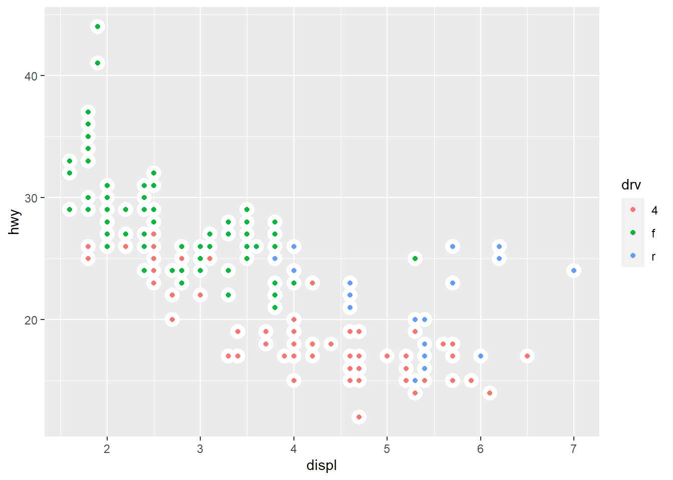
3.7 Exercises
1. What is the default geom associated with
stat_summary()? How could you rewrite the previous plot to
use that geom function instead of the stat function?
I assume this is what the authors mean by previous plot:
ggplot(data = diamonds) +
  stat_summary(
    mapping = aes(x = cut, y = depth),
    fun.min = min,
    fun.max = max,
    fun = median
  )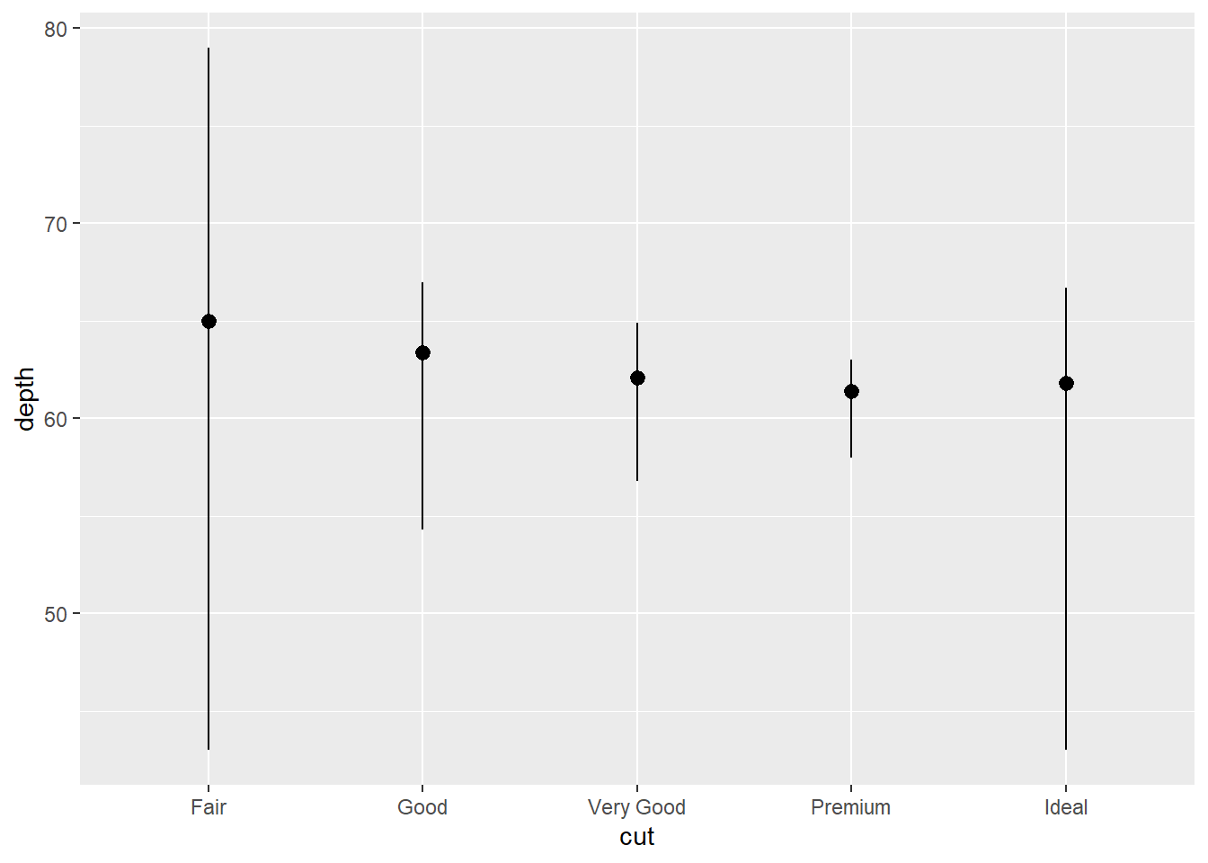
The documentation available by ?stat_summary shows that
geom = "pointrage". The documentation
for?geom_pointrange reads that it is various ways of
representing vertical interval defined by x,
ymin, and ymax. So here is what we can write
using the geom_pointrange() instead of the
stat_summary() function:
ggplot(data = diamonds) +
  geom_pointrange(
    mapping = aes(x = cut, y = depth),
    stat = "summary",
    fun = median,
    fun.min = min,
    fun.max = max
  )
2. What does geom_col() do? How is it different to
geom_bar()?
There are two types of bar charts: geom_bar() and
geom_col(). geom_bar() makes the height of the
bar proportional to the number of cases in each group (or if the weight
aesthetic is supplied, the sum of the weights). If you want the heights
of the bars to represent values in the data, use geom_col()
instead. geom_bar() uses stat_count() by
default: it counts the number of cases at each x position.
geom_col() uses stat_identity(): it leaves the
data as is.
3. Most geoms and stats come in pairs that are almost always used in concert. Read through the documentation and make a list of all the pairs. What do they have in common?
The following table is a list of all the pairs I compiled. There was
a lesson from DataCamp that
covered this question. Also, this site contains list
of all geom_ and stat_ functions available in
ggplot2.
| Geom_ | Stat_ | Common Description |
|---|---|---|
geom_bar(), geom_col() |
stat_count() |
Bar charts |
geom_bin2d() |
stat_bin2d() |
Heatmap of 2d bin counts |
geom_boxplot() |
stat_boxplot() |
A box and whiskers plot (in the style of Tukey) |
geom_contour(),
geom_contour_filled() |
stat_contour(),
stat_contour_filled() |
2D contours of a 3D surface |
geom_count() |
stat_sum() |
Count overlapping points |
geom_density() |
stat_density(), |
Smoothed density estimates |
geom_density_2d() |
stat_density_2d() |
Contours of a 2D density estimate |
geom_dotplot() |
stat_bindot() |
Dot plot |
geom_function() |
stat_function() |
Draw a function as a continuous curve |
geom_hex() |
stat_bin_hex() |
Hexagonal heatmap of 2d bin counts |
geom_freqpoly(),
geom_histogram() |
stat_bin() |
Histograms and frequency polygons |
geom_qq(),
geom_qq_line() |
stat_qq(),
stat_qq_line() |
A quantile-quantile plot |
geom_quantile() |
stat_quantile() |
Quantile regression |
geom_sf() |
stat_sf() |
Visualize sf objects |
geom_smooth() |
stat_smooth() |
Smoothed conditional means |
geom_violin() |
stat_violin() |
Violin plot |
4. What variables does stat_smooth() compute? What
parameters control its behaviour?
Try running ?stat_smooth() on your R console.
stat_smooth() computes the following variables: -
y or x: Predicted value - ymin or
xmin: Lower pointwise confidence interval around the mean -
ymax' orxmax: Upper pointwise confidence interval around the mean -se`:
Standard error
The parameters controlling the behavior of
stat_smooth(): - method: Smoothing method
(function) to use, accepts either NULL or a character
vector. - formula: Formula to use in smoothing function. -
se: display confidence interval around smooth
(TRUE by default) - na.rm: If
FALSE, the default, missing values are removed with a
warning. If TRUE, missing values are silently removed. -
orientation: The orientation of the layer. -
show.legend: NA, the default, includes if any
aesthetics are mapped. - method.args: List of additional
arguments passed on to the modelling function defined by
method.
5. In our proportion bar chart, we need to set group = 1. Why? In other words what is the problem with these two graphs?
ggplot(data = diamonds) +
  geom_bar(mapping = aes(x = cut, y = after_stat(prop)))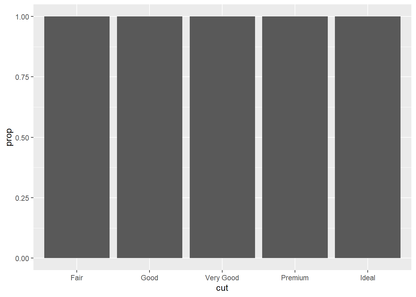
ggplot(data = diamonds) +
  geom_bar(mapping = aes(x = cut, fill = color, y = after_stat(prop)))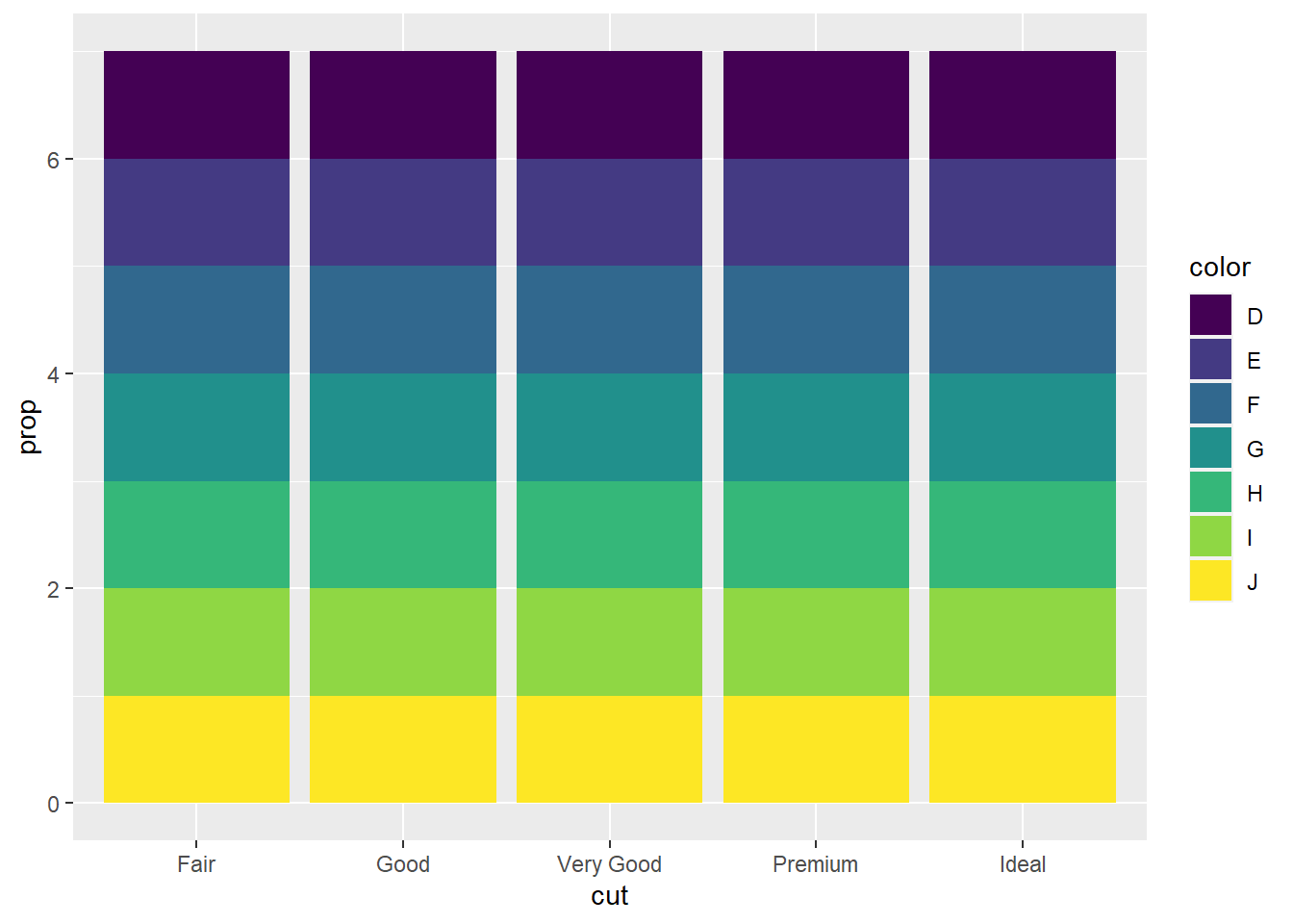
As you can see from the outpu graphs, without group = 1,
all the bars end up with the same height. This is because the
geom_bar() function assumes that the groups are equal to
the x values since the stat computes the counts within the
group.
Note: Read about ?after_stat() function.
prop refers to percent of points in that panel in the
position.
Here is the intended bar graph:
ggplot(data = diamonds) +
geom_bar(mapping = aes(x = cut, y = after_stat(prop), group = 1))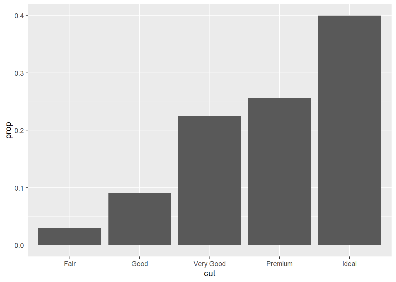 Next section (3.8) explains how you can fill the bars with colors.
3.8 Exercises
1. What is the problem with this plot? How could you improve it?
ggplot(data = mpg, mapping = aes(x = cty, y = hwy)) +
  geom_point()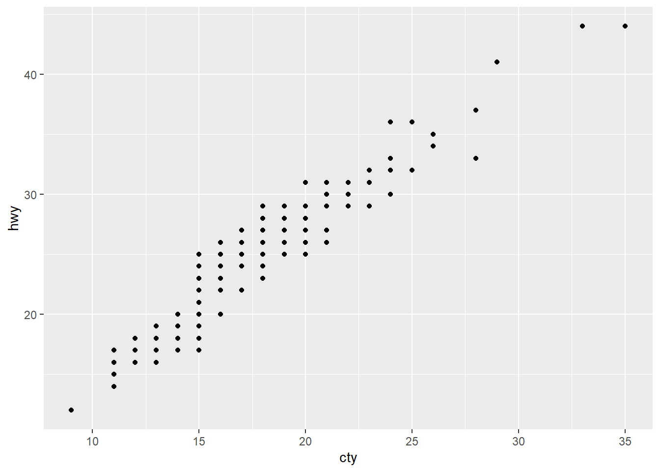
Try running dim(mpg). There should be 234 points on this
graph, so we know the problem is that points over being over-plotted. We
would need to adjust the position of the points.
Setting position = "jitter" fixes this problem.
ggplot(data = mpg, mapping = aes(x = cty, y = hwy)) +
  geom_point(position = "jitter")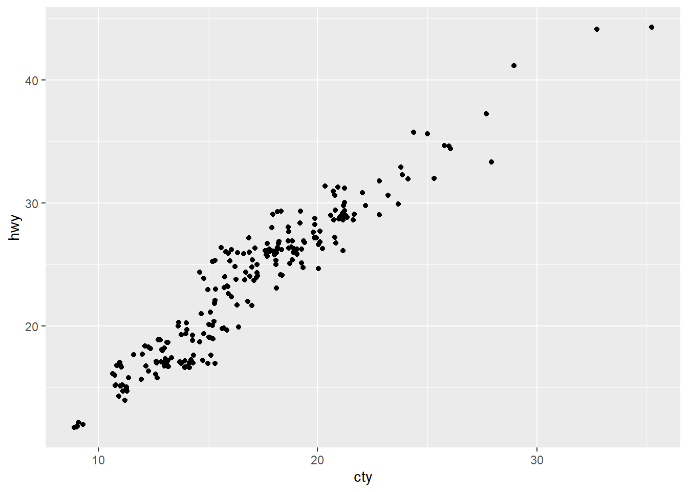
2. What parameters to geom_jitter() control the amount
of jittering?
?geom_jitter() shows two parameters that control the
amount of jittering. The width controls the amount of
horizontal displacement, and height controls the amount of
vertical displacement. You can play around by assigning different values
to the two parameters.
ggplot(data = mpg, mapping = aes(x = cty, y = hwy)) +
  geom_jitter(width = 0)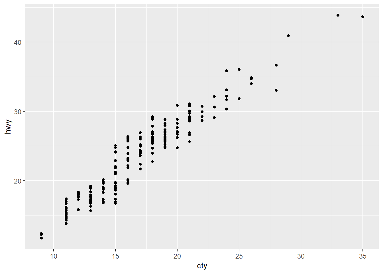
ggplot(data = mpg, mapping = aes(x = cty, y = hwy)) +
  geom_jitter(height = 0)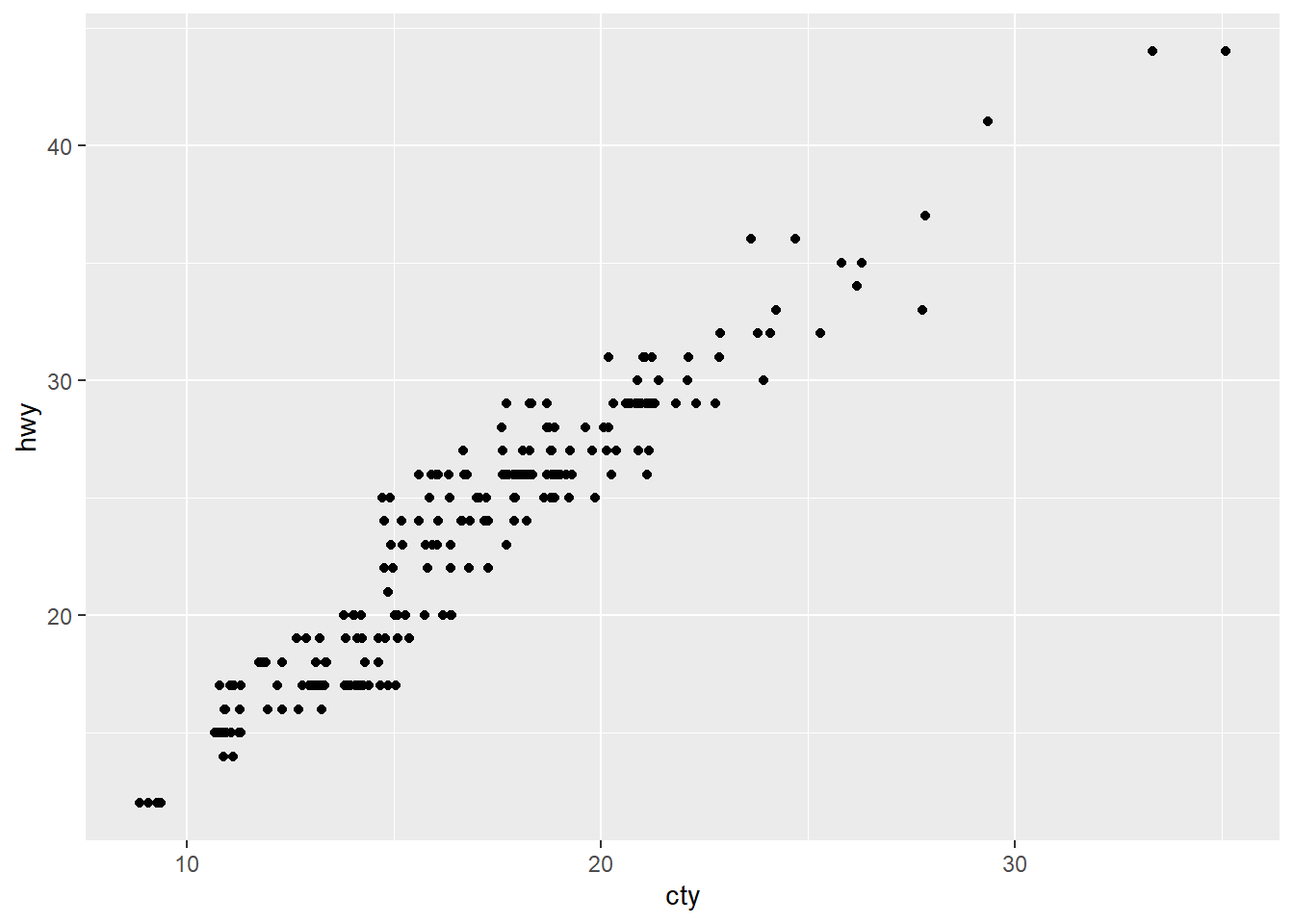
ggplot(data = mpg, mapping = aes(x = cty, y = hwy)) +
  geom_jitter(width = 20)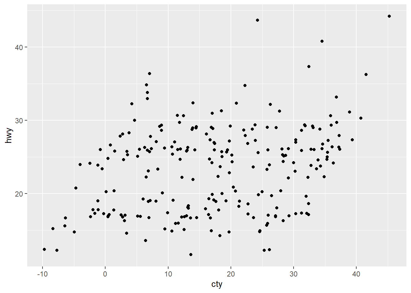
ggplot(data = mpg, mapping = aes(x = cty, y = hwy)) +
  geom_jitter(height = 20)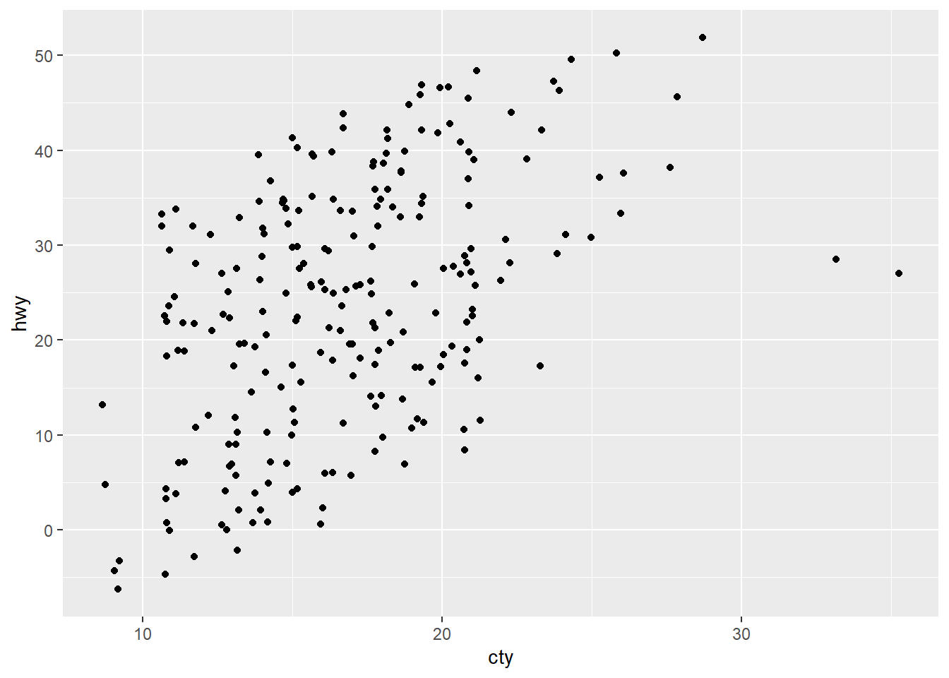
Note that if you assign 0s to both height and
width, the resulting graph will be identical to the one
made using geom_point().
ggplot(data = mpg, mapping = aes(x = cty, y = hwy)) +
  geom_jitter(height = 0, width = 0)
3. Compare and contrast geom_jitter() with
geom_count().
geom_jitter() adds a small amount of random variation to
th location of each point. It is a useful way of handling overplotting
caused by discreteness in smaller datasets.
geom_count() counts the number of observations at each
location, then maps the count to point area. It is also useful when you
have discrete data and overplotting issue. Unlike
geom_jitter(), geom_count() is able to create
different size of the points relative to the number of observations.
ggplot(data = mpg, mapping = aes(x = cty, y = hwy)) +
  geom_jitter()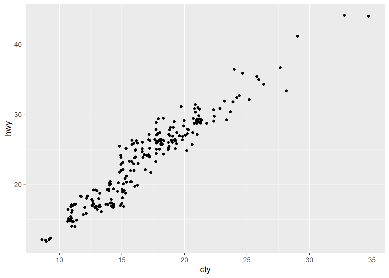
ggplot(data = mpg, mapping = aes(x = cty, y = hwy)) +
  geom_count()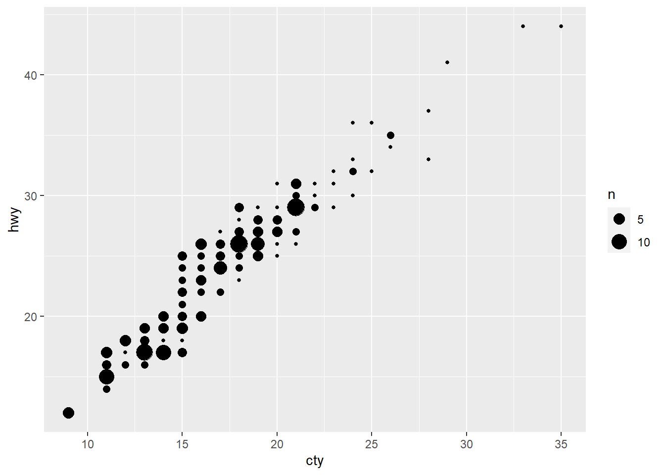
With the mpg dataset, we see that
geom_count() is starting to cause the problem of
overplotting again.
We can play around with the color.
ggplot(data = mpg, mapping = aes(x = cty, y = hwy, color = class)) +
  geom_jitter()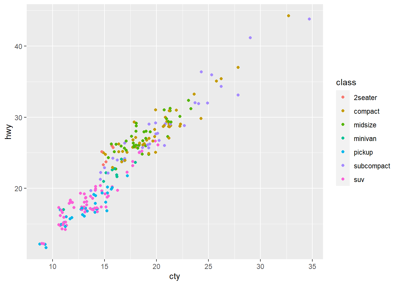
ggplot(data = mpg, mapping = aes(x = cty, y = hwy, color = class)) +
  geom_count()
ggplot(data = mpg, mapping = aes(x = cty, y = hwy, color = class)) +
  geom_count(position = "jitter")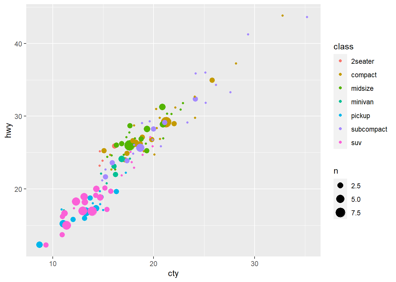
While the graphs did add an additional info of class,
none of the graphs seems to solve the overplotting issue.
4. What’s the default position adjustment for
geom_boxplot()? Create a visualisation of the
mpg dataset that demonstrates it.
?geom_boxplot() shows that the default position
adjustment is dodge2. Here is the r code from the previous
problem, but using geom_boxplot() instead:
ggplot(data = mpg, aes(x = cty, y = hwy, color = class)) +
  geom_boxplot()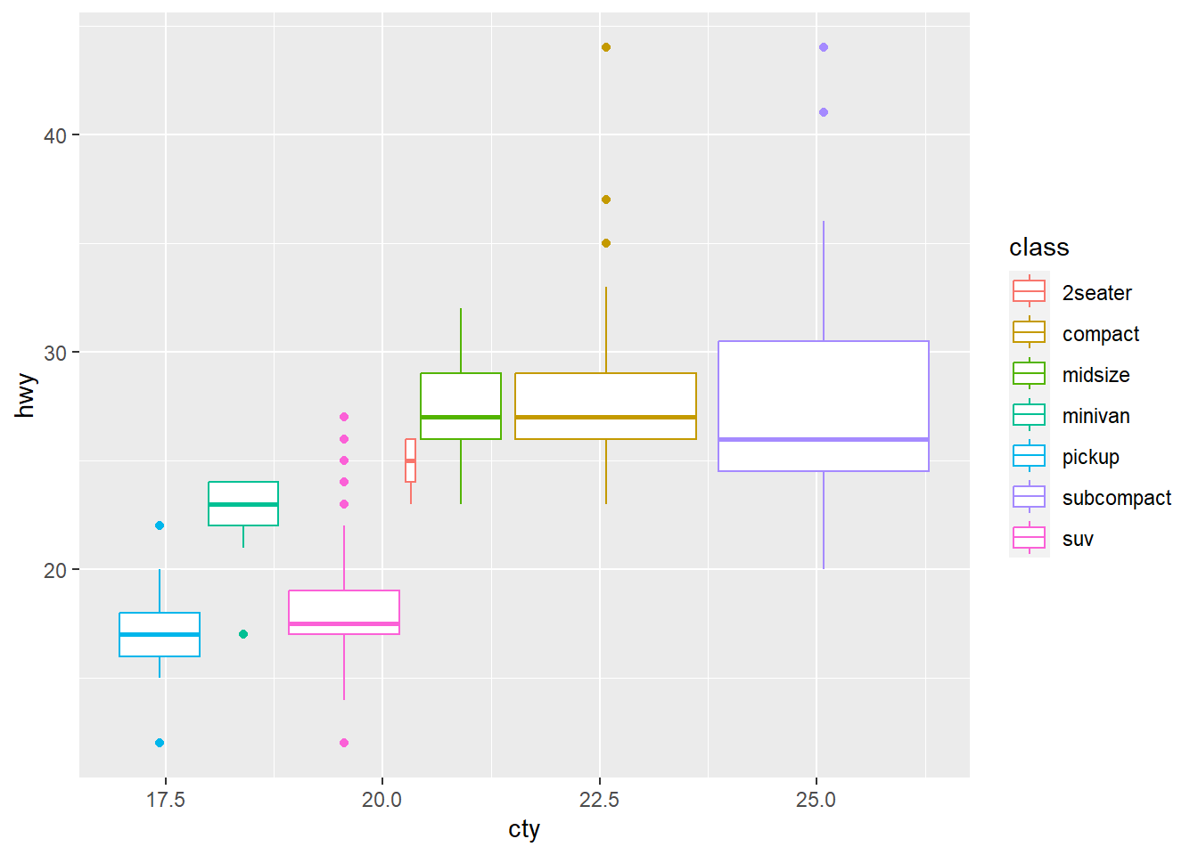
3.9 Exercises
1. Turn a stacked bar chart into a pie chart using
coord_polar().
Start with a stacked bar chart:
ggplot(mpg, aes(x = factor(1), fill = drv)) +
  geom_bar()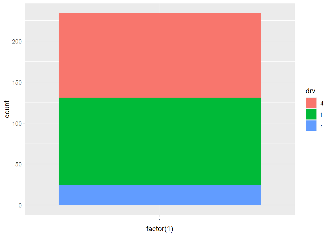
Add coord_polar(theta="y") to create pie chart:
ggplot(mpg, aes(x = factor(1), fill = drv)) +
  geom_bar(width = 1) +
  coord_polar(theta = "y")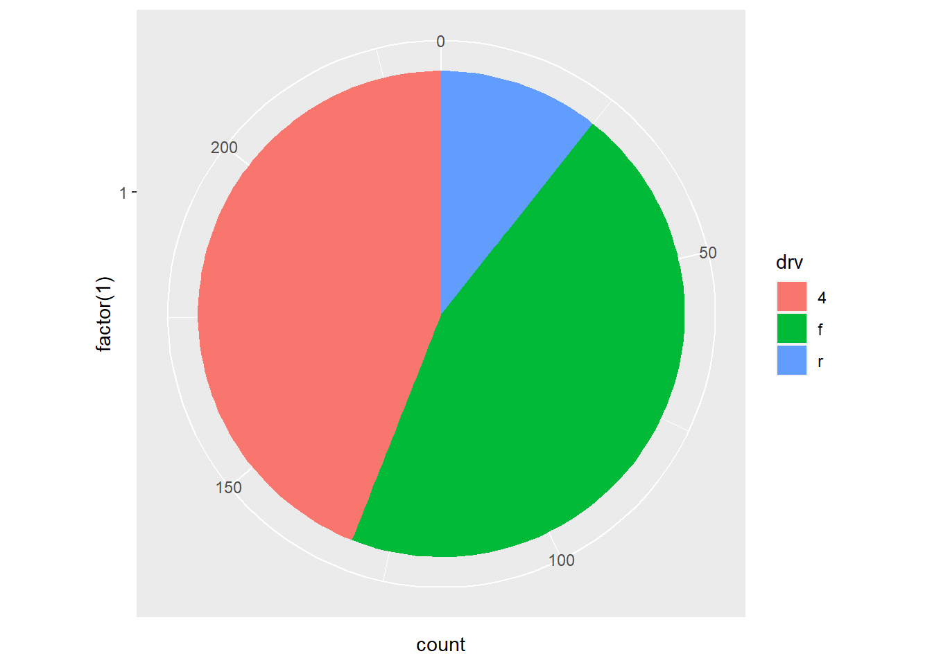
2. What does labs() do? Read the documentation.
The labs() allows you to add axis titles, plot titles,
and a caption to the plot. I have been using it since the very beginning
of this chapter.
Note that labs is not the only way to add titles. Other
functions such as xlab(), ylab(),
ggtitle() can also be used.
3. What’s the difference between coord_quickmap() and
coord_map()?
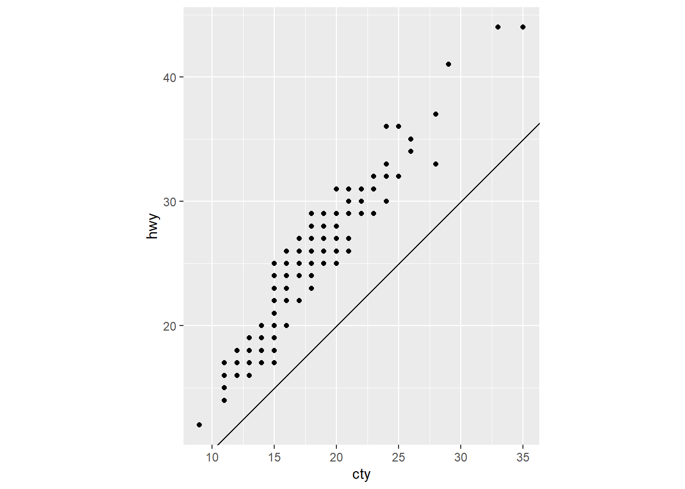
4. What does the plot below tell you about the relationship between
city and highway mpg? Why is coord_fixed() important? What
does geom_abline() do?
ggplot(data = mpg, mapping = aes(x = cty, y = hwy)) +
  geom_point() +
  geom_abline() +
  coord_fixed()